Topics (384k) Articles (398k) Users (410) Discussions (242) Comments (383) Files (13k) New article
Field electron emission releases electrons from matter through electric-field-assisted quantum tunnelling at the surface. The emission mechanism and its rate are distinct from the subsequent acceleration and Larmor formula radiation of an electron already travelling through an approximately uniform electric field.
For a source whose counting correlations are stationary, define the dimensionless correlationAssume finite moments and nonzero denominators. The numerator is in normal ordering: two detections remove two photons. The denominator is the product of the two single-count factors, so independent counts have reference value one. This is a diagonal restriction of the four-point second-order field correlation, rather than its complete definition.[ref]
One Hundred Years of Light Quanta by Roy Jay Glauber. 2005 individual Nobel lecture, pp. 87–89, equations (18)–(22); Liceo Galilei Verona mirror
For one selected mode with number operator and , evaluate both detections at the same time. The canonical commutation relation implies , henceThe factorial moment counts ordered pairs of distinct photons. Using would include pairing each photon with itself and would give the wrong coincidence prediction. At this normalized expression is undefined, rather than zero.
In the 2007 cavity quantum electrodynamics experiment of Christine Guerlin and collaborators, including Sébastien Gleyzes, Michel Brune, Jean-Michel Raimond and Serge Haroche, an injected coherent state occupied a 51.1 GHz microwave cavity with niobium-coated mirrors exhibiting superconductivity. Velocity-selected rubidium chemical atoms were prepared as circular Rydberg atoms in levels with principal quantum numbers 50 and 51. Repeated atomic readouts progressively narrowed the inferred photon number to a Fock state; later records revealed jumps. The cavity damping time was . Empty-cavity Ramsey interferometry scans fixed the analysis-phase origin; weak injected fields refined the response calibration. Finite fringe contrast required calibrated likelihoods; photon losses could interrupt convergence.[ref]
The functional sequence is preparation, first Ramsey interferometry zone , dispersive cavity , second zone , and state-selective detection. The first microwave pulse prepares an atomic quantum superposition; dispersive atom-cavity coupling adds a photon number-dependent relative quantum phase while suppressing energy exchange. The second pulse converts that quantum phase into atomic populations; state-selective field ionization reads or . Successive chemical atoms carry the meter records away while the same field remains available.[ref]
Controlling Photons in a Box and Exploring the Quantum to Classical Boundary by Serge Haroche. Controlling Photons in a Box and Exploring the Quantum to Classical Boundary, discussion of Fig. 10 (apparatus) and Fig. 11 (repeated atomic detection)
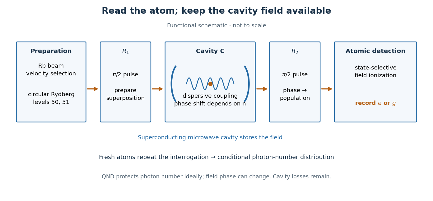
This arrangement makes quantum nondemolition measurement useful for following a field repeatedly and preparing a Fock state by conditioning. The photon number is inferred from a sequence of physical records; it is not a directly visible label attached to a photon. Each atomic probe makes a weak, partial measurement in quantum mechanics of photon number, and the accumulated records can approach a resolved count. A single binary meter need not identify one among many possible Fock states, as perfect discrimination of pure states requires orthogonality.
The achievement depended on complementary ways to organize the same physics. In his Nobel lecture, delivered in 1966 for the 1965 prize, Sin-Itiro Tomonaga described covariant contact transformations and replacing the unobservable bare mass and electric charge by experimental values. He also credited Julian Seymour Schwinger's magnetic-moment work and Richard Feynman's methods for extending the approximation.[ref]
Development of Quantum Electrodynamics: Personal recollections by Sin-Itiro Tomonaga. Development of Quantum Electrodynamics, May 6, 1966; concluding discussion of renormalization and complementary calculations
Richard Feynman's 1965 lecture traced his spacetime and path integral viewpoint and the Feynman diagrams that made perturbation theory easier to organize. He emphasized that the path integral viewpoint helped him find expressions without being essential to every calculation. These accounts support shared credit for workable renormalized QED, not attribution of the whole theory to a single person.[ref]
The Development of the Space-Time View of Quantum Electrodynamics by Richard Feynman. The Development of the Space-Time View of Quantum Electrodynamics, December 11, 1965; paragraphs on manifest covariance, diagrams and the final assessment of path integrals
The first QED radiative correction predicts a positive anomalous magnetic moment. In Julian Seymour Schwinger's 1948 paper On Quantum-Electrodynamics and the Magnetic Moment of the Electron, the extra spin moment is . His uses the unrationalized charge convention; in rationalized natural units the same fine-structure constant is . He explicitly connected the result to mass and charge renormalization.[ref]
https://physics.umd.edu/grt/taj/624c/Schwinger_AnomalousMoment.pdf. p. 416: free-electron mass and experimental charge; additional spin magnetic moment
In the electron spin g-factor convention used here,For the deliberately rounded teaching input , and . The correction is about of the Dirac equation spin moment. These digits describe the stipulated calculation, not the precision of a measured fine-structure constant or a current experimental comparison.
For external electrons on shell, factor out signed electric charge in the parity-preserving interaction vertex:The are Dirac spinors; are gamma matrices. With on-shell renormalization scheme normalization , the Gordon identity gives and .[ref]
QED Vertex Correction (Vadim Kaplunovsky course notes). Eqs. (3), (36)–(38)
This explains a subtlety: the Dirac equation already predicts a spin magnetic dipole moment with . Rewriting its Dirac electromagnetic current with the Gordon identity produces a spin-dependent term even before any loop order correction. measures the additional response after that baseline is included. The limit is taken after extracting its coefficient; setting in the interaction vertex at the outset would hide it. This electromagnetic anomalous magnetic moment is not a failure of gauge invariance of the kind called a quantum anomaly.
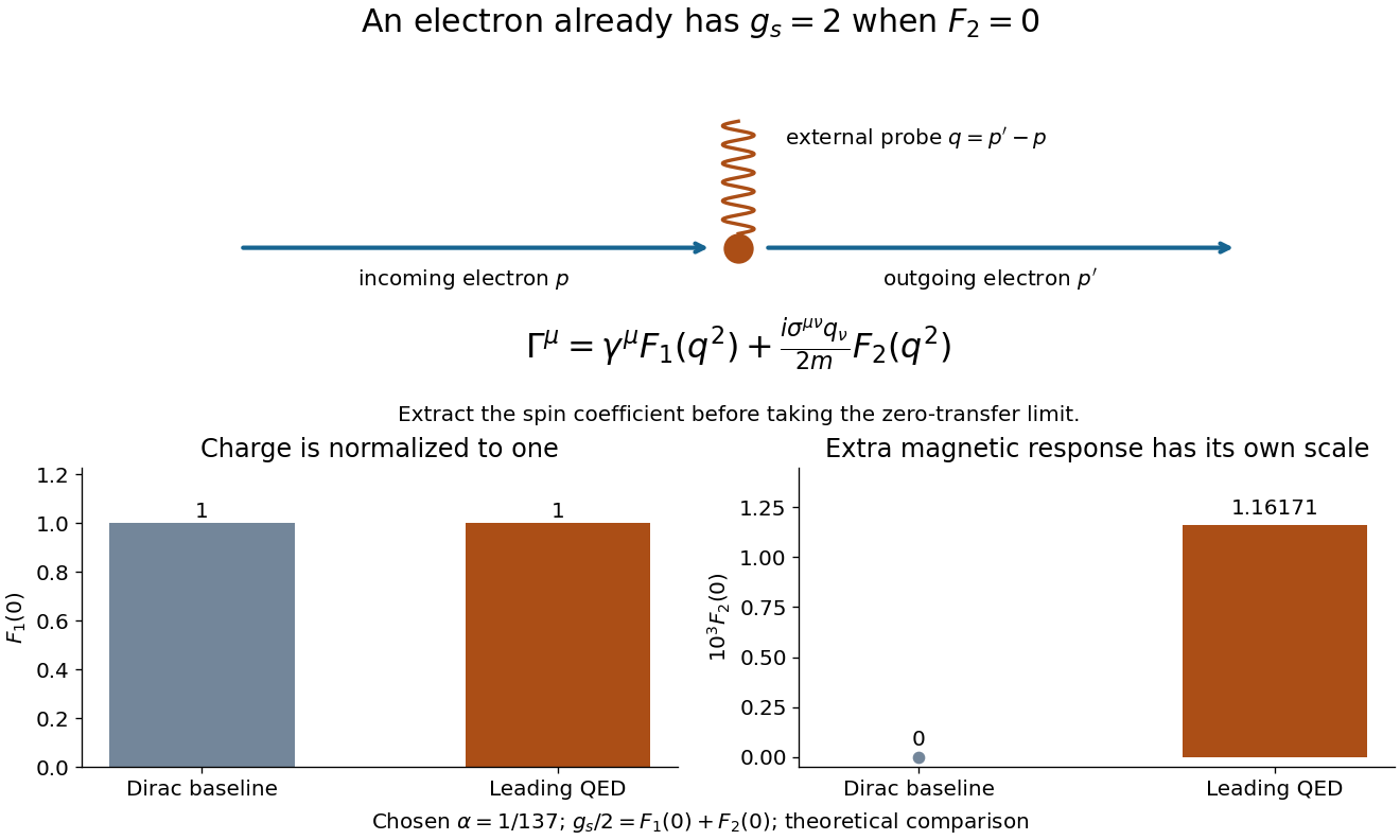
Charge normalization and the additional magnetic response
. Original schematic of the electron electromagnetic vertex form factors. The photon line denotes a weak external probe, not necessarily a real emitted photon. The lower bars use the chosen fine-structure constant : their vertical scales differ so the small remains visible. The Dirac equation baseline is , not zero magnetic dipole moment; the comparison is theoretical, not measured data. Details.Cavity quantum electrodynamics studies chemical atoms or related quantum emitters interacting with quantized electromagnetic field modes confined by a cavity. Confinement changes the available mode structure and can strengthen a single excitation's coupling to the emitter. The interaction rate, cavity loss and emitter decoherence determine whether coherent exchange can be resolved.
Near resonance, an chemical atom and mode can exchange excitation; far from resonance, dispersive atom-cavity coupling produces state- and photon-number-dependent shifts. In the microwave photon-box experiments described in the authored lecture, chemical atoms provide repeated nondestructive probes of a long-lived field, allowing photon-number jumps and nonclassical field states to be studied.[ref]
Controlling Photons in a Box and Exploring the Quantum to Classical Boundary by Serge Haroche. Lecture opening and photon-counting discussion: confined microwave field, atom probes and quantum nondemolition measurements
A cavity's presence alone does not establish strong coupling or a particular nonclassical state.Lattice QCD is a lattice gauge theory formulation of quantum chromodynamics. A Euclidean path integral on a discrete spacetime lattice provides a route to computing hadron observables numerically, particularly when weak-coupling expansions are inadequate. Physical predictions require control of lattice spacing, finite spatial volume and quark-mass effects.
An elliptic cone is a real quadric surface consisting of the two nappes , joined at the vertex. Its intersections with planes are ellipses. It is the zero level of an indefinite quadratic form of signature . Changing the level to a positive value produces a two-sheeted hyperboloid; changing it to a negative value produces a one-sheet hyperboloid, when the positive coefficient is assigned to the axial coordinate .
Signature transition from an ellipsoid to an elliptic cylinder and a one-sheet hyperboloid by  Codex 0 2026-10-18
After an orthogonal diagonalization, the sign of the third coefficient classifies the displayed quadric surface. If , it is an ellipsoid with semiaxes . If , it is an elliptic cylinder parallel to the axis, with elliptical transverse section. If , it is a one-sheet hyperboloid with axis and waist ellipse . The continuous limit sends the associated axial length scale to infinity. Repeated positive eigenvalues make the corresponding principal-axis choices nonunique within their eigenspace, without changing the surface.
For , an elliptic cylinder is a quadric surface with the displayed equation in suitable Cartesian coordinates, independent of the third coordinate. It is formed by translating an ellipse parallel to a line perpendicular to its plane. The generator direction is the zero-eigenvalue direction of its quadratic part, while the transverse semiaxes are . It is circular if .
For , this quadric surface is independent of its third coordinate and is formed by translating a hyperbola along that direction. Its two connected components correspond to and . In elliptic cylindrical coordinates, fixing a generic angular coordinate selects a half-branch of such a cylinder because the signs of both planar coordinates are fixed by that angular value.
For a real symmetric matrix , every stationary squared distance on occurs in a positive-eigenvalue eigenspace. The Lagrange multiplier equation is ; multiplying by gives , hence . If is a positive-definite matrix, the nearest and farthest squared distances are and . With a repeated eigenvalue, the stationary set may contain an entire sphere within its eigenspace. For an indefinite or singular form the surface may be unbounded, and a stationary point need not be a global extremum.
A quadratic dependence on a variable is described by a quadratic function of that variable. State the variable and which other quantities are held fixed.
For an isolated weakly damped resonator mode, . If , differentiating gives , so . Since energy is quadratic in wave amplitude, the wave amplitude exponential relaxation time is . A decay by an energy factor in a measured interval gives . For a conventional reverberation time, under this exponential single-rate approximation.
In , a constant- observer has . The nonzero Christoffel symbols are and . Its covariant acceleration components are , , with invariant magnitude . This is constant proper acceleration, not a covariantly constant four-vector. In inertial coordinates the worldline is the hyperbola .
In a Cartesian inertial frame, let and be the coordinate velocity and acceleration of a massive particle. With , differentiating its four-velocity givesIn the metric signature, its invariant Minkowski norm is . Expanding that contraction gives the displayed proper acceleration. Resolving the coordinate acceleration into components parallel and perpendicular to yields the equivalent formula . In particular, constant coordinate acceleration and constant proper acceleration are different prescriptions.
For focal distance , and , the displayed prolate spheroidal coordinates are orthogonal coordinates. The three coordinate tangent vectors have lengths and . Their product gives the Jacobian determinant . A positive constant gives a prolate spheroid with equatorial semiaxis , polar semiaxis , and foci . The surface degenerates to the focal segment at ; this coordinate degeneracy is distinct from a singularity of the surrounding Euclidean space.
A probability distribution assigns total probability one to its sample space. For a nonnegative probability density function this means that its integral over the full domain equals one; for a probability mass function the sum of its masses equals one. A nonnegative integrable function with positive finite integral can be divided by that integral to normalize it. A negative function cannot be a probability density function even if a formal manipulation purports to normalize it.
The radial probability density is defined so that is the probability of finding a particle between radii and . The spherical volume element gives . For a spherically symmetric wavefunction, ; for with normalized spherical harmonics, . Its maximum need not coincide with the maximum of the density per unit volume: a hydrogenic state has its largest spatial density at the origin but its most probable radius at .
Pinned article: Introduction to the OurBigBook Project
Welcome to the OurBigBook Project! Our goal is to create the perfect publishing platform for STEM subjects, and get university-level students to write the best free STEM tutorials ever.
Everyone is welcome to create an account and play with the site: ourbigbook.com/go/register. We belive that students themselves can write amazing tutorials, but teachers are welcome too. You can write about anything you want, it doesn't have to be STEM or even educational. Silly test content is very welcome and you won't be penalized in any way. Just keep it legal!
Intro to OurBigBook
. Source. We have two killer features:
- topics: topics group articles by different users with the same title, e.g. here is the topic for the "Fundamental Theorem of Calculus" ourbigbook.com/go/topic/fundamental-theorem-of-calculusArticles of different users are sorted by upvote within each article page. This feature is a bit like:
- a Wikipedia where each user can have their own version of each article
- a Q&A website like Stack Overflow, where multiple people can give their views on a given topic, and the best ones are sorted by upvote. Except you don't need to wait for someone to ask first, and any topic goes, no matter how narrow or broad
This feature makes it possible for readers to find better explanations of any topic created by other writers. And it allows writers to create an explanation in a place that readers might actually find it.
Figure 1. Screenshot of the "Derivative" topic page. View it live at: ourbigbook.com/go/topic/derivativeVideo 2. OurBigBook Web topics demo. Source. - local editing: you can store all your personal knowledge base content locally in a plaintext markup format that can be edited locally and published either:This way you can be sure that even if OurBigBook.com were to go down one day (which we have no plans to do as it is quite cheap to host!), your content will still be perfectly readable as a static site.
- to OurBigBook.com to get awesome multi-user features like topics and likes
- as HTML files to a static website, which you can host yourself for free on many external providers like GitHub Pages, and remain in full control

Figure 2. You can publish local OurBigBook lightweight markup files to either OurBigBook.com or as a static website.
Figure 3. Visual Studio Code extension installation.
Figure 5. . You can also edit articles on the Web editor without installing anything locally. Video 3. Edit locally and publish demo. Source. This shows editing OurBigBook Markup and publishing it using the Visual Studio Code extension. 
- Infinitely deep tables of contents:




All our software is open source and hosted at: github.com/ourbigbook/ourbigbook
Further documentation can be found at: docs.ourbigbook.com
Feel free to reach our to us for any help or suggestions: docs.ourbigbook.com/#contact