Topics (384k) Articles (398k) Users (410) Discussions (242) Comments (383) Files (13k) New article

Suppose a calibrated measurement bounds the fractional loss of a nonzero superconducting persistent current by , with , over a duration . Take by choosing the circulation direction. Under the constant-, constant-, undriven RL circuit model,The inequality follows because the logarithm is increasing. The final approximation requires and slightly understates the exact upper bound. If is uncertain, an independently established upper bound on gives the conservative electrical resistance bound. The uncertainty in the initial reading, the final reading, background subtraction and drift must all be included in ; a display resolution alone does not provide it.
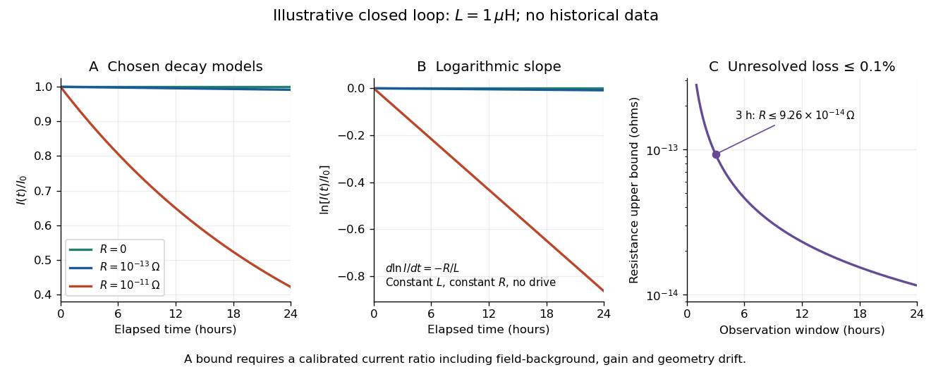
An illustrative exponential decay, its logarithmic slope and the resulting resistance bound
. Chosen numerical model, not historical data: fixed self-inductance and no external drive. The final panel assumes a calibrated fractional-loss bound of at each chosen observation duration. Longer observation tightens the bound only while that fractional uncertainty remains controlled. Details.For an original illustrative example, let and suppose the corrected electric current ratio after is at least . ThenThese are conditional bounds for stipulated parameters, not values attributed to the 1914 apparatus. With the same but , the model instead gives and : a readily visible loss on the chosen scale.
A resolved decay can be checked using its logarithm:A straight line supports this constant-parameter model; curvature or jumps demand a different account. If an effective electrical resistance varies with time while remains fixed and the loop remains undriven, only its time average is constrained:This does not bound every instantaneous value of . Changing self-inductance or external linked magnetic flux adds terms to the circuit equation, so an uncorrected magnetic signal cannot simply be substituted for . Nonobservation of decay leaves arbitrarily small positive constant electrical resistance compatible with a finite observation: it is not a logical proof that .
The apparatus and motivating measurement are described in permanganate-iron titration; the following is an original account of its possible errors. Assume correct titrant standardization, the acidic permanganate-iron balance, quantitative conversion of the sampled , and additive contributions expressed as equivalent titrant volumes. WriteHere is the sample titre, the titration blank, background reagent consumption, and signed offsets of the observed titration endpoints from the respective stoichiometry conditions after background consumption. The subscripts distinguish sample and blank. is additional sample-specific permanganate demand, absent from the blank; is apparent delivery used to fill an initially air-containing burette tip rather than enter the flask. Assume the blank's tip is already filled; the sample should also have after proper preparation. These terms are a diagnostic model, not measured components of the stipulated blank.
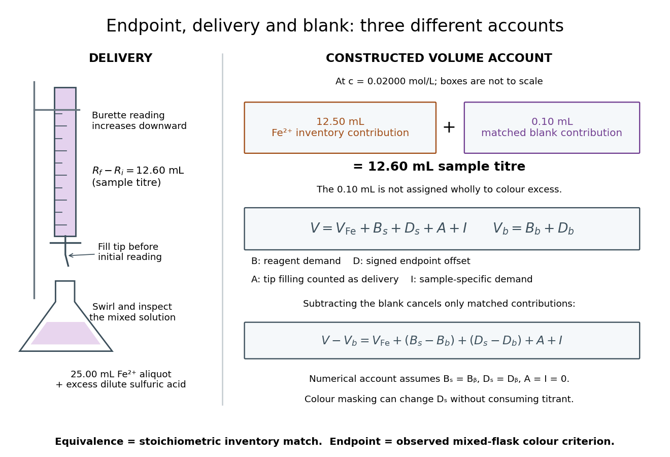
Subtracting the two accounts proves the error relationThe simple inference is valid when this residual is negligible. Matching water and sulfuric acid tests the background terms, but does not by itself establish : flask composition and viewing conditions can differ. A coloured sample can mask residual permanganate, changing the assigned titration endpoint without a corresponding redox consumption. A sample-specific reducing agent instead contributes positive by consuming permanganate. A reagent titration blank cannot measure either effect just by omitting the sample.
A transient purple streak before mixing is not the mixed-flask titration endpoint. Conversely, the equivalence point is the five-to-one inventory match, without a promised visible flag. In the ideal selective model, a persistent excess colour requires some permanganate beyond that match. No particular drop size, waiting time or endpoint offset is stipulated here; the same stated colour criterion must be applied to sample and blank, and its transferability checked.
The model also predicts error direction. If a tip bubble disappears during sample delivery, makes the inferred amount of substance too high because final minus initial burette reading includes liquid that stayed in the tip. Conditioning the tip before the first reading prevents this particular discrepancy; subtracting a separate titration blank is not an instrument repair. Repeated aliquots test scatter, a known added inventory tests the five-to-one response, and an independent titrant standardization tests . These are the proposed controls from permanganate-iron titration, with distinct diagnostic roles; none alone proves absence of all sample interference.
Relativistic dust is a continuum of noninteracting massive particles with one local four-velocity and negligible pressure. With signature , and rest mass density , its stress-energy tensor has the displayed form. Contracting stress-energy conservation with and using metric compatibility gives . Substituting back yields wherever : each particle follows a geodesic. The cosmological pressureless matter model is a homogeneous application.
Consider an original idealized narrow-band model for one matched spatial mode and one polarization of waves. In the classical Rayleigh-Jeans law regime, an available thermal power can be written , where is the effective bandwidth and the equivalent input noise temperature. Assume a linear detector with stable positive gain and absorb its bandwidth, Boltzmann constant and response factor into . Then the output is , with input-referred receiver noise temperature . These are model assumptions, not a reconstruction of the historical electronics.
Two references with known noise temperatures giveso the two-load radiometer calibration yieldsSubtracting the reference equations eliminates the unknown receiver term; substituting back determines it. An arbitrary stable output offset can likewise be eliminated from the interpolation for , although separating that offset from then requires additional information.
For deliberately chosen inputs, set , , and . These are equivalent noise temperatures; physical load thermometry must be converted consistently at the observing frequency. The reference outputs are and . A sky-input output gives . If independent estimates assign to atmosphere, to antenna loss and to ground pickup in this lumped additive model, the residual is .
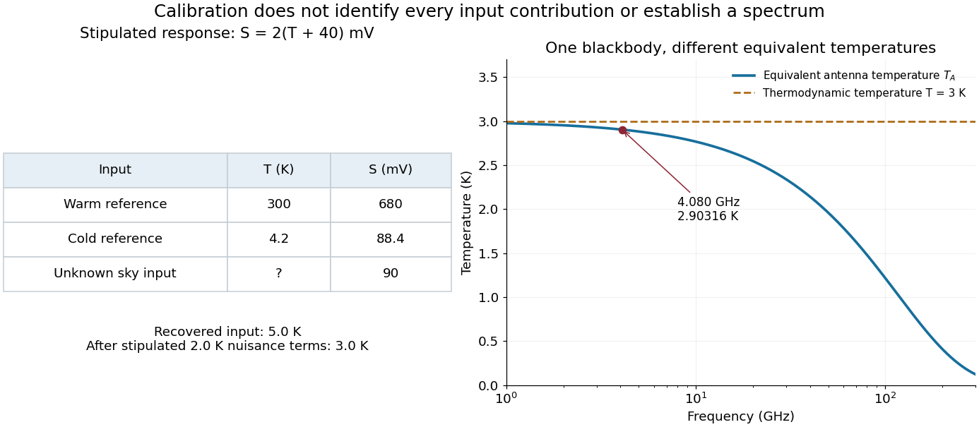
Original calibration arithmetic and the distinction between an antenna temperature and a thermodynamic temperature
. Chosen reference temperatures, receiver response and additive contributions; none are fitted historical measurements. The final panel calculates the Rayleigh-Jeans law equivalent antenna temperature of a stipulated blackbody. A change in frequency changes that equivalent temperature even though the underlying thermodynamic temperature is fixed. Details.The subtraction exposes what a noise budget must achieve. A error in the assigned atmospheric term becomes a error in the residual, even with exact detector calibration. Multiplicative attenuation requires a different correction: if an isothermal atmosphere has transmission , its ideal contribution is in the same classical equivalent-temperature convention. Recovering then requires both subtracting atmospheric emission and dividing by . The additive toy budget applies when its terms already refer to the same receiver input.
There is also a conditioning issue. If is small, a fixed output error strongly changes the inferred temperature. Widely separated reference temperatures improve the scale determination only if the receiver remains linear over that range; measuring the reference repeatedly tests stability rather than proving linearity. The experiment therefore motivates a model, a calibration and a set of independent checks, each with its own assumptions.
Assume future null geodesic completeness. The compactness of the future horismos of a trapped surface makes a nonempty compact achronal boundary without edge. Projection along a complete timelike vector field into the Cauchy hypersurface is injective, open by invariance of domain, and closed by compactness. Connectedness forces surjectivity, contradicting the noncompact Cauchy hypersurface. This global step completes the contradiction.[ref]
Gravitational Collapse and Space-Time Singularities by Roger Penrose. p. 59, compactness and noncompactness contradiction
The Null Raychaudhuri equation is the light-ray version of the Raychaudhuri equation associated with Amal Kumar Raychaudhuri. His original work concerned relativistic cosmology.[ref]
Amal Kumar Raychaudhuri by Jayant Vishnu Narlikar. research discussion, PDF pp. 4–6, the 1955 paper Relativistic Cosmology
For the normal null geodesic congruence before its first focal point, null twist vanishes. With an affine parameter , the four-dimensional equation reduces to the displayed ordinary differential equation. The null shear contraction is nonnegative on the transverse screen space, and the null convergence condition makes the other part of nonnegative. Consequently .For , put . ThenA regular negative null expansion therefore cannot persist beyond if the null geodesic extends that far. The null focusing theorem turns this estimate into a focal-point bound. The number refers to an affine parameter, not the proper time of a light ray, which is zero.
For an original soluble model, prescribe constant along one twist-free beam; this does not specify an entire solution of the Einstein field equations. Introduce a positive affine scale and the dimensionless variablesFor an infinitesimal area define before the first zero. Since , where primes now mean , the same model becomesTwo independently checkable solutions areThe nonnegative extra focusing term moves the first zero earlier. Direct substitution into both ordinary differential equations verifies the solutions; numerical integration of the nonlinear equation provides a separate comparison with the linear beam equation.
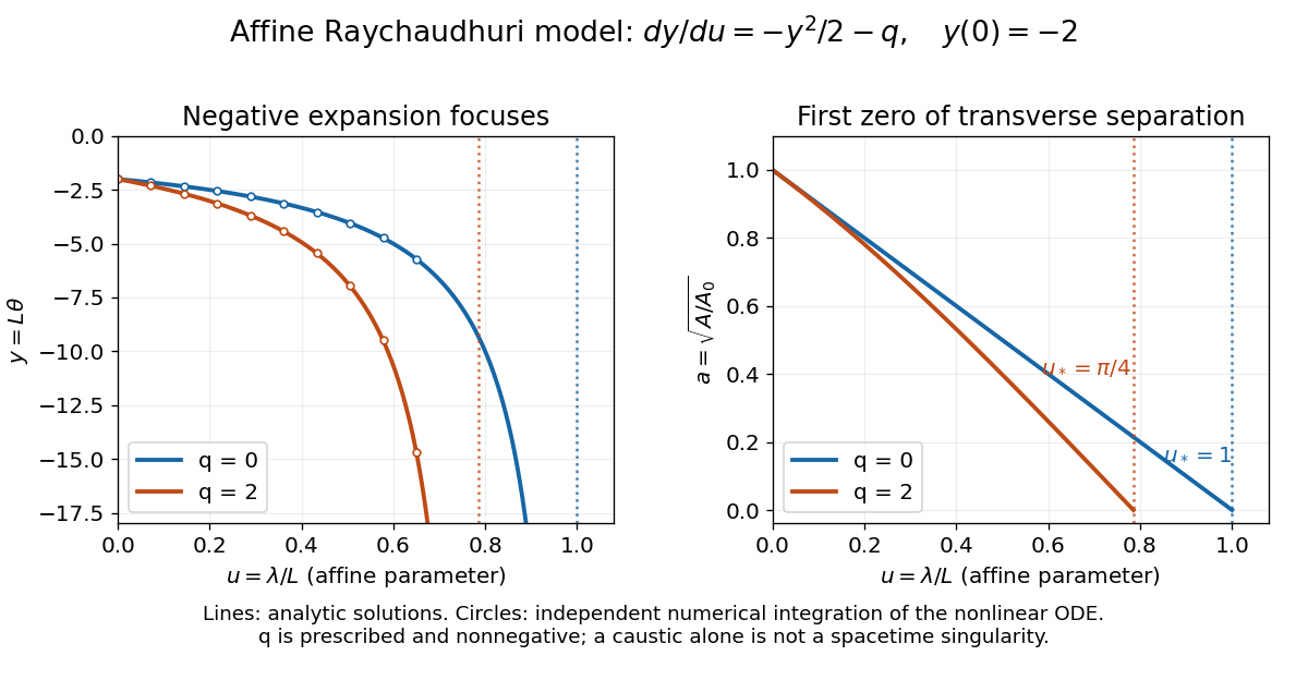
Finite affine focusing in two explicitly defined Raychaudhuri models
. Both beams start with . Curves show the exact solutions for and ; circles independently integrate . The first zeros occur at and , respectively. These are illustrative ordinary differential equation models, not fitted collapse data. Details.A focal point makes this beam description degenerate, but individual null geodesics may continue smoothly through it. Even converging light in Minkowski spacetime can form a caustic. Converting local focusing into null geodesic incompleteness requires the global step below.
A concrete example separates a trapped surface from a failure of coordinates. Use geometrized units , metric signature , and the regular ingoing Eddington-Finkelstein coordinates of a Schwarzschild black hole with mass :For a round sphere, choose future null vector normalsThe spherical null expansion in ingoing coordinates follows directly from : . At , ; at , it is . Both future light fronts shrink in the second case. At , , so this sphere is marginally outer trapped surface, not a strict trapped surface. In the spherical model this boundary is an event horizon; that identification does not extend to arbitrary geometries.
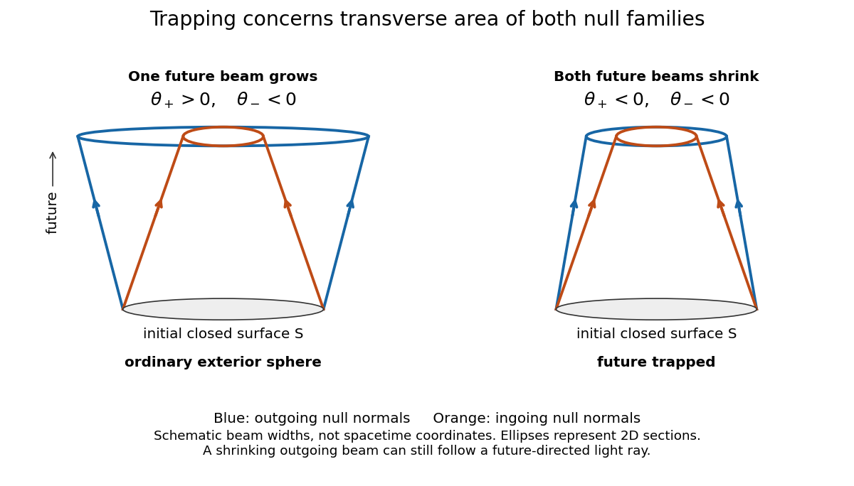
Both future null families contract at a trapped surface
. The schematic compares signs of null expansion. The horizontal separation represents transverse beam width, not a radial spacetime coordinate; the ellipses represent two-dimensional sections. No horizon location or endpoint of a null geodesic is encoded by the drawing. Details.Although is affine as written, generally obeys . These are valid initial normals for the sign test; use affine rescaling of a null normal before applying the affine Null Raychaudhuri equation. Regularity of the displayed metric tensor at shows why a divergence in another chart would not establish null geodesic incompleteness.
On a compact trapped surface, both null expansions have a uniform negative margin. Sufficiently small smooth perturbations controlling the relevant metric tensor and surface derivatives preserve trapping. This conditional robustness does not prove that every nonspherical gravitational collapse creates a trapped surface.[ref]
Gravitational Collapse and Space-Time Singularities by Roger Penrose. p. 58, small departures from symmetry
Hans Georg Dehmelt describes a , Penning trap, with positive ring and negative endcaps apart. Axial RF emission tracked an injected seven-electron bunch losing particles; reducing the drive retained the last electron. A weak magnetic bottle converted spin changes into axial-frequency changes. At successive probe frequencies, counted spin flips traced a resonance.[ref]
Experiments with an isolated subatomic particle at rest by Hans Georg Dehmelt. Dehmelt, pp. 584–589, Figs. 1, 3, 6–7; Columbia scan
The inference can be explained without inventing a detector calibration. Let a weak bottle have on-axis field . The magnetic dipole potential energy adds to the axial harmonic oscillator potential energy, soA change in the magnetic dipole moment therefore shifts the monitored axial angular frequency. This is a simplified readout model, not a quantitative reconstruction of the historical bottle. It illustrates how a transition in one degree of freedom becomes a detectable change in another.
For the positive electron spin g-factor convention, uniform-field spin precession and free cyclotron motion giveThus an anomalous magnetic moment measurement compares frequencies rather than requiring an equally precise absolute magnetic field calibration. The free must first be inferred from trapped motion with the necessary corrections. A spin-flip count versus probe frequency supplies evidence for a transition resonance; it does not directly measure a spatial electron radius. Nor is this radio readout an optical fluorescence record: different experiments require different preparations and detectors. In a precision comparison, repeat scans with changed drive strength and monitor magnetic field drift, motional excitation and detector back-action; these are experimental-design checks, not additional historical observations asserted here.
Define positive angular frequency magnitudes and , with uniform , . Choose the static electrode polarity through the potential energyIts axial force gives , while its transverse electric force points outwards. For , let . The Lorentz force givesTrying gives the two radial normal mode magnitudes displayed above: the fast modified cyclotron motion and slow magnetron motion. For the rotation directions reverse. Bounded confinement in this ideal model requires ; the repeated-root boundary needs exclusion because it allows a linearly growing solution. At large , and .
The ideal identitiesfollow directly from that quadratic. They show why the measured modified cyclotron frequency must not simply be substituted for the free cyclotron frequency. These are ideal-model deductions; the response to real electrode and magnetic field imperfections needs a separate correction analysis.
Thermoelectric cooling uses the Peltier effect to remove heat from a load using electrical work. A typical thermoelectric module connects many pairs of different semiconductors electrically in a series circuit and thermally in parallel between two faces. For an idealized pair with , positive conventional current crosses n to p at the cold bridge and p to n at the hot return. With common bridge material and isothermal contacts, the intervening metal contributions telescope: the net pair coefficient is . For identical pairs define the module Seebeck coefficient .
Choose fixed face temperatures , , module electrical resistance and open-circuit thermal conductance . All three module parameters are constants over the chosen operating range. Positive is the orientation absorbing Peltier effect heat at c. Define as net heat extracted from the cold reservoir per unit time, as net heat delivered to the hot reservoir per unit time, and as electrical power entering the module. Despite the conventional letters , both denote power in watts, not accumulated energy. Ferrotec gives the corresponding single-stage equations and distinguishes module performance from bypass leaks.[ref]
An actual institutional protocol is CTU's Measurement of characteristics of a Peltier cell. Its cooling run uses a water container, an insulating cap and a current-limited supply; both face temperatures are recorded every minute while electric current is monitored. The apparatus includes a water-cooled exchanger, copper blocks and brass containers. The heating run resets the water near room temperature before reversing polarity. The handout specifies no thermometer type and reports no dataset. Its modular junction geometry is shown separately from the external thermal assembly.[ref]
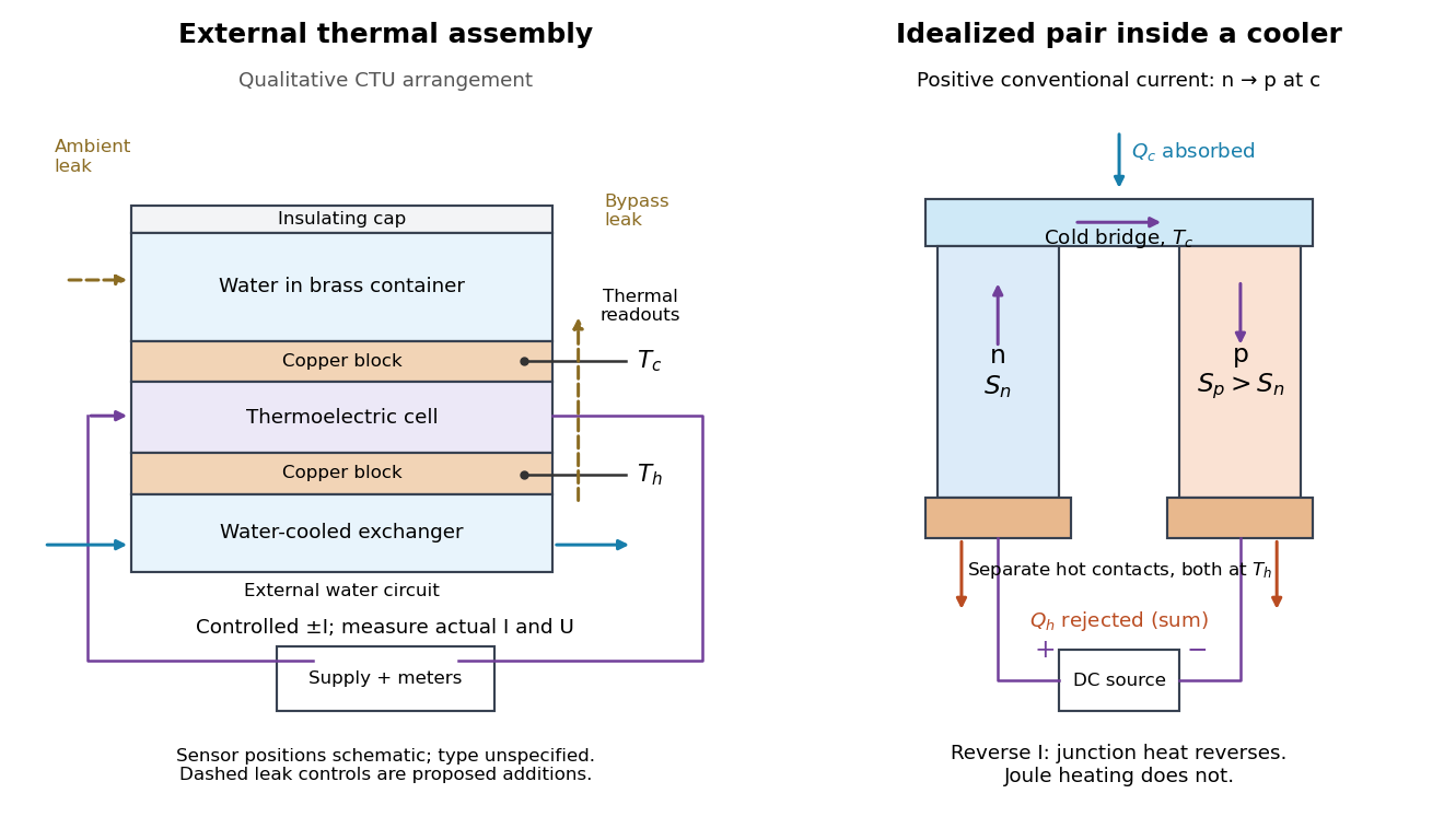
The following is a proposed quantitative extension. Keep the physical face labels fixed throughout reversal: c denotes the observed object's side and h the exchanger side, even if their actual temperatures change order. Use an independently read thermometer at each thermal contact and log the actual signed electric current and terminal electric potential difference. Maintain reproducible contact pressure and contact layers. A sensor in water measures water temperature, which need not equal the face temperature during a transient; verify mixing and contact equilibration before using it as a face reading. Do not interchange sensor leads when reversing the supply.
The strongest separation compares runs at the same , water mass, contact conditions and environment, rather than subtracting arbitrary final temperatures. One option is short initial-rate runs after resetting the whole assembly to a reproducible state. Define as the net power entering the monitored object, inferred from its calibrated effective heat capacity and initial temperature slope. In a simple symmetric model, let include background heat transfer at that state and the dissipated power reaching the object. Thenwhere in the thermoelectric cooling model below. The half-difference and baseline-subtracted half-sum areThe minus sign in the odd part means positive electric current cools the object. The even part has to subtract the zero-current baseline: otherwise heat conduction and ambient exchange remain mixed with Joule heating. Independently measured heat capacity is essential for converting a thermal slope into watts; include the blocks, container and water that actually equilibrate on the measurement timescale.
Useful controls are zero-current drift at several matched temperature differences, equal-magnitude positive and negative electric currents, and repetition of a sequence such as with thermal resets. A calibrated small heater on the object can test the heat capacity and lost-heat correction independently. Check Joule heating in supply leads and contacts, bypass heat conduction through supports and wiring, and ambient convection and thermal radiation. Insulation reduces a leak; it does not establish that it is zero. Measure terminal power at the module boundary so lead losses are not mistaken for module heating.
An odd thermal response supports a reversible current-coupled contribution, but does not by itself locate all of it at one junction: the Thomson effect in nonuniform leads can also be odd. Sensor offsets, unequal current magnitudes, drifting thermal contacts and different junction temperatures during the two runs can contaminate both parts. In particular, heating proportional to is even only when the compared electrical resistance is the same. CTU's qualitative reversal illustrates switching heating and cooling; the matched-state controls above would be needed for a coefficient measurement.
At uniform temperature, define the material Peltier coefficient by transported heat current along positive conventional current:Its units are . In one dimension, , with electric current density and thermal conductivity . Here heat excludes the electrochemical potential contribution to total energy flux.[ref]
Now orient positive conventional current from material A into material B, at a common junction temperature . Define as heat taken from the junction's thermal surroundings. The outgoing transported heat minus the incoming transported heat givesThe local released heat is . Authors defining a junction coefficient by released heat therefore use the opposite sign. Exchanging A and B reverses the coefficient; reversing at fixed A and B reverses the junction's thermal response. An individual material coefficient and a junction difference are different quantities.
For an original stipulated example, choose and at . The Kelvin thermoelectric relation gives , . A positive flowing A to B absorbs . A separate junction electrical resistance would dissipate for either direction. If all that dissipation heats the junction, its net absorbed power is forwards and backwards. These numbers illustrate a chosen thermal accounting boundary, not measured material data or a universal allocation of contact heating.
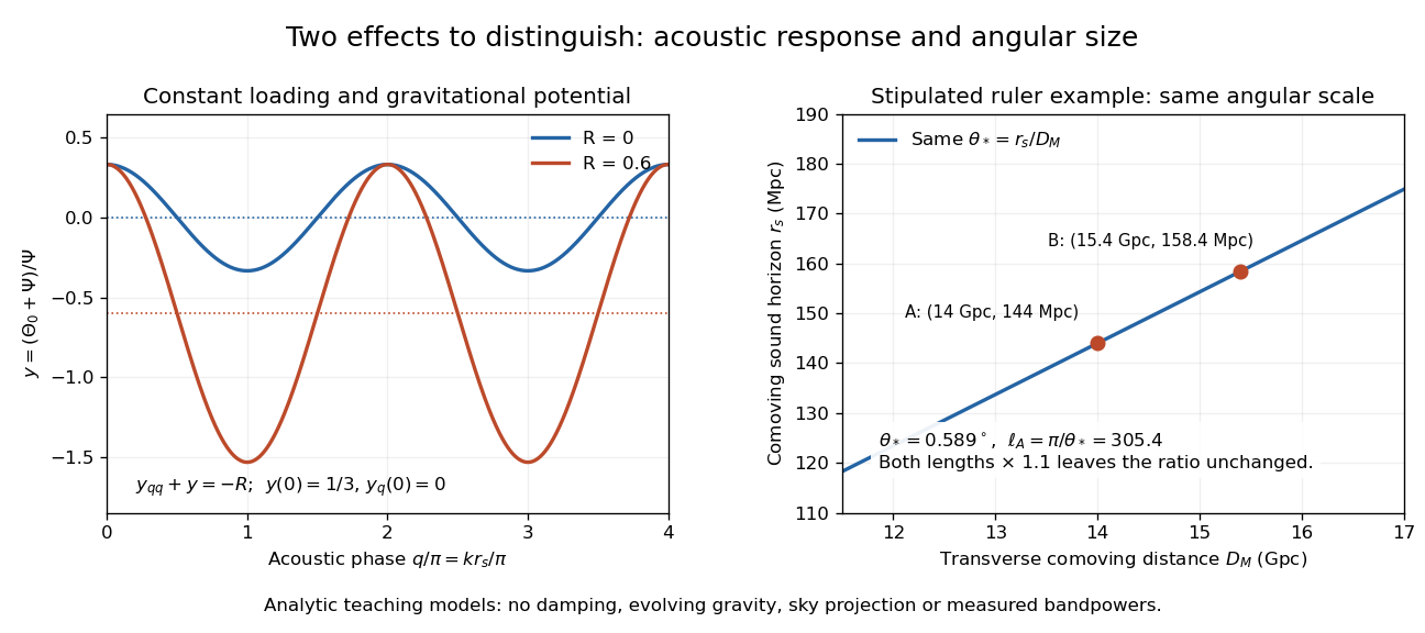
A deliberately restricted forced harmonic oscillator shows two effects of the baryon loading parameter without duplicating the full photon Boltzmann hierarchy. Use conformal time in seconds, a comoving wavenumber in inverse metres, constant , and equal constant dimensionless Newtonian gauge gravitational potentials . The energy densities and use the same units. Neglect expansion drag, Silk damping and evolution of the potentials. The photon-baryon sound speed is . Writing for the photon monopole temperature perturbation, the photon-baryon acoustic oscillator reduces toFor this gives the displayed forced equation. Constant loading and the neglected expansion drag make this a local teaching model, not a self-consistent expanding cosmology with fixed forever.
Choose and , the static matter-era Sachs-Wolfe combination normalized by . With , direct substitution givesAt , successive extrema have equal magnitudes . At the stipulated , whereas . The shifted equilibrium makes alternating extrema unequal. This is an elementary illustration of how the baryon loading parameter changes acoustic amplitudes; these extrema are neither measured peak heights nor a complete Cosmic microwave background power spectrum. Comparing curves at fixed isolates the response; at fixed and , increasing also reduces the photon-baryon sound speed and hence the phase.
For example, holding gives sound horizons at and at . Their ratio is . Each term of the forced equation has units of inverse seconds squared because and are dimensionless and is an inverse time. In the actual photon-baryon fluid, grows with the scale factor and the sound horizon is the integral of the evolving photon-baryon sound speed.
In the small-parameter regime, the slow coordinate describing Paul trap secular motion approximately obeys a harmonic oscillator equation at angular frequency . Its superposed fast motion is Paul trap micromotion. Substituting the leading fast displacement from the RF-averaged trapping potential gives the displayed expression in our phase convention. A small positional ripple can have substantial velocity, because differentiating it brings down the large angular frequency . Precision spectroscopy must therefore address both Paul trap secular motion and Paul trap micromotion; merely obtaining a bounded trajectory does not eliminate Doppler shifts.
The slow part of a trapped trajectory in the small-parameter regime of a Paul trap. Its angular frequency is approximately set by the curvature of the RF-averaged trapping potential, including any static electric potential contribution. Paul trap micromotion is superposed on this slow motion.
Write the RF electric field as , where is a real peak-amplitude vector with a common drive phase. Decompose the trajectory into a slow position and fast displacement . Over one short RF cycle, hold fixed. The leading fast equation and solution areThe homogeneous slow part is absorbed into . Expand the electric field to first order in and average, using :The second equality uses zero curl in the quasistatic RF electric field. This derives an effective potential energy, not an extra static electric potential. Its dependence confines either sign of electric charge towards a field-amplitude minimum. Using an RMS field instead would give a coefficient multiplying .
The approximation needs fast displacement small compared with the field's variation length and slow angular frequencies small compared with . In the stated electric quadrupole model, small and of order provide a controlled regime, away from stability boundaries. Add when . For the result isFor the pure RF case, . The square-root condition describes leading local restoring curvature; it is not a substitute for full Mathieu equation stability. Collisions, departures from the ideal electric quadrupole, and a displaced RF null require further analysis.
Specify the convention before quoting a stability parameter. Choose the ideal, rotationally symmetric electric potentialHere is a static voltage coefficient, is a peak RF voltage coefficient, is the length entering this displayed normalization, is mass, is signed electric charge, and is the drive angular frequency. The coefficient is neither a peak-to-peak voltage nor an RMS voltage. An apparatus's ring-to-cap voltage requires matching its electrode surfaces to this electric potential; electrode radius alone does not define our . The minus sign fixes the RF phase at .
With , Newton's second law gives a Mathieu equation for each Cartesian coordinate :Thus a three-dimensional Paul trap needs simultaneous bounded solutions in all three directions. Changing the sign of reverses and shifts the RF phase by half a cycle; it does not change the ideal infinite-time stability regions. Rescaling the voltage or length convention changes the numerical parameters. Floquet theory determines stability of the full Mathieu equation; the small-parameter approximation below does not establish stability for arbitrary . Bounded mathematical motion can still hit an electrode if its amplitude exceeds the available space.
On , , with infinite exterior potential, separation of variables gives the normalized eigenbasisThe boundary values vanish and the functions are orthonormal. A general state is a superposition of these products. A degenerate energy eigenspace can contain nonseparable linear combinations of products at the same energy, so a single separated product is not the most general stationary wavefunction in that eigenspace.
For a real central potential and the outgoing convention , the Partial-wave S-matrix is . The cosine form of the Jacobi-Anger expansion fixes and for . Comparing the outgoing part of each phase-shifted radial cosine with the incident plane wave gives the displayed scattering amplitude. Integrating gives the displayed scattering cross-section, since the constant angular mode has squared norm and each positive-order cosine has squared norm . Reversing the multiplicities would already fail to reproduce the free plane wave at zero scattering phase shift.
Pinned article: Introduction to the OurBigBook Project
Welcome to the OurBigBook Project! Our goal is to create the perfect publishing platform for STEM subjects, and get university-level students to write the best free STEM tutorials ever.
Everyone is welcome to create an account and play with the site: ourbigbook.com/go/register. We belive that students themselves can write amazing tutorials, but teachers are welcome too. You can write about anything you want, it doesn't have to be STEM or even educational. Silly test content is very welcome and you won't be penalized in any way. Just keep it legal!
Intro to OurBigBook
. Source. We have two killer features:
- topics: topics group articles by different users with the same title, e.g. here is the topic for the "Fundamental Theorem of Calculus" ourbigbook.com/go/topic/fundamental-theorem-of-calculusArticles of different users are sorted by upvote within each article page. This feature is a bit like:
- a Wikipedia where each user can have their own version of each article
- a Q&A website like Stack Overflow, where multiple people can give their views on a given topic, and the best ones are sorted by upvote. Except you don't need to wait for someone to ask first, and any topic goes, no matter how narrow or broad
This feature makes it possible for readers to find better explanations of any topic created by other writers. And it allows writers to create an explanation in a place that readers might actually find it.
Figure 1. Screenshot of the "Derivative" topic page. View it live at: ourbigbook.com/go/topic/derivativeVideo 2. OurBigBook Web topics demo. Source. - local editing: you can store all your personal knowledge base content locally in a plaintext markup format that can be edited locally and published either:This way you can be sure that even if OurBigBook.com were to go down one day (which we have no plans to do as it is quite cheap to host!), your content will still be perfectly readable as a static site.
- to OurBigBook.com to get awesome multi-user features like topics and likes
- as HTML files to a static website, which you can host yourself for free on many external providers like GitHub Pages, and remain in full control

Figure 2. You can publish local OurBigBook lightweight markup files to either OurBigBook.com or as a static website.
Figure 3. Visual Studio Code extension installation.
Figure 5. . You can also edit articles on the Web editor without installing anything locally. Video 3. Edit locally and publish demo. Source. This shows editing OurBigBook Markup and publishing it using the Visual Studio Code extension. 
- Infinitely deep tables of contents:




All our software is open source and hosted at: github.com/ourbigbook/ourbigbook
Further documentation can be found at: docs.ourbigbook.com
Feel free to reach our to us for any help or suggestions: docs.ourbigbook.com/#contact