The relative refractive index of medium two with respect to medium one is $n_{21}=n_2/n_1$, using their absolute refractive indices at the same frequency. For transparent media with isotropy and positive refractive indices, Snell's law gives $n_{21}=\sin i/\sin r$, with the angles measured from the interface normal. Thus a refraction measurement in air directly determines an index relative to air. Converting it to an absolute refractive index requires the refractive index of that air; replacing it by one is an approximation.

For a plane wave proportional to $e^{i(N\omega z/c-\omega t)}$, the complex refractive index separates phase propagation from attenuation. In a nonmagnetic medium $N^2={ϵ}_r$, so $n^2-{\kappa }^2={ϵ}_r^{\prime }$ and $2n\kappa ={ϵ}_r^{\prime \prime }$. The passive branch has $\kappa \ge 0$. If $\kappa \ll n$ and ${ϵ}_r^{\prime }>0$, then $n\simeq \sqrt{{ϵ}_r^{\prime }}$ and $\kappa \simeq {ϵ}_r^{\prime \prime }/(2\sqrt{{ϵ}_r^{\prime }})$. These signs assume the $e^{-i\omega t}$ convention for the complex permittivity.

MIT's documented slotted-line waveguide measurement shorts one end of a rectangular electromagnetic waveguide and excites it through a probe coupled by capacitance. A second such probe moves through a longitudinal slot, aligned with the wall electric current to reduce disturbance. Its output locates axial standing wave nulls. The book's standing-wave setup chooses a frequency above the first waveguide cutoff frequency and below higher-mode cutoffs. Lowering it below the first cutoff instead reveals spatial decay away from the source. The text supplies apparatus and an observable comparison, rather than a table of measured null positions.^[ref]

The inference can be checked without assuming that detector output is proportional to electric field amplitude. At fixed measured frequency, record several minima at coordinates $z_0,\dots ,z_N$; then estimate ${\lambda }_g=2(z_N-z_0)/N$ when the minima are consecutive. This uses positions alone. Compare the result with the guided wavelength prediction using independently measured $a$ and $f$. The $40\mathrm{mm}$ spacing above is a synthetic example, not a reading from the MIT apparatus.

Additional proposed controls are to keep probe insertion fixed, repeat the scan in both directions, recheck source frequency, and compare shallow probe settings for shifts in the minima. These test probe loading, mechanical backlash and drift. A deliberately reflecting termination supplies the standing wave; varying its position should translate the pattern without changing adjacent-null spacing in a uniform single-mode region. Source-adjacent evanescent waves, unintended reflections, additional propagating normal modes, detector noise and finite positional resolution can spoil that inference. A disappearing remote signal alone does not distinguish below-cutoff decay from loss or poor excitation, and a scan at one frequency does not measure a pulse's group velocity.

The guided wavelength is the distance for a $2\pi$ change of axial wave phase in a propagating normal mode. For the vacuum-filled rectangular electromagnetic waveguide,for ${\mathrm{TE}}_{10}$, with ${\lambda }_0=c/f$ and $f>f_c$. It exceeds the vacuum wavelength at the same frequency. This longer axial spacing is consistent with $v_{\mathrm{ph}}>c$: multiplying ${\lambda }_g$ by $f$ gives the phase velocity, not the group velocity.

Two oppositely traveling fields at the same frequency form a standing wave. For a perfect electric short at $z=0$, the total electric field is proportional to $\sin (\beta z)\sin (\pi x/a)$, so successive axial electric nodes are separated byThus neighboring minima in a slotted line scan give half a guided wavelength. In the original $a=30\mathrm{mm}$, $f=1.25f_c$ example, $d=40\mathrm{mm}$ implies ${\lambda }_g=80\mathrm{mm}$, not $40\mathrm{mm}$. Combined with the chosen $f$, the inferred broad dimension is $a={\lambda }_0/[2\sqrt{1-({\lambda }_0/{\lambda }_g{)}^2}]=30\mathrm{mm}$. Below cutoff, $\beta$ is imaginary and $2\pi /\beta$ is not a physical periodic spacing.

In a hollow rectangular electromagnetic waveguide with perfect conductor walls and axis $z$, a transverse magnetic polarization has $B_z=0$ and a nonzero longitudinal electric field $E_z$. The wall boundary conditions impose $E_z=0$ around the transverse rectangle. Separation of variables therefore gives $E_z=E_0\sin (n\pi x/a)\sin (m\pi y/b)e^{i(k_{z}z-\omega t)}$, with $n,m\ge 1$. Setting either index to zero makes the entire field vanish. Thus there is no ${\mathrm{TM}}_{n0}$ or ${\mathrm{TM}}_{0m}$ branch. The transverse eigenvalue is $k_{\perp }^2=(n\pi /a{)}^2+(m\pi /b{)}^2$, with dispersion relation ${\omega }^2/c^2=k_z^2+k_{\perp }^2$. This exclusion is specific to this geometry and these boundary conditions.

The University of Colorado Boulder's Lab 3: Filters, §§7.1–7.4, specifies measuring the resistor and capacitor, then driving the assembled RC low-pass filter with a function generator. A two-channel oscilloscope reads actual input and output using high electrical impedance. Sweep the frequency, record the voltage amplitude ratio, and locate $1/\sqrt{2}$. A control compares a cable with a $10\times$ oscilloscope probe on a resistive voltage divider, isolating measurement capacitance before using the probe for the filter. A slow square wave then lets discharge timing estimate the time constant independently. Agreement supports the RC low-pass frequency response; source output impedance, probe loading, and instrument signal bandwidth limit it. These are prescribed measurements, with no measured dataset supplied here.^[ref]

The two-channel setup can also test the predicted phase difference directly: for positive frequency $f$, measure the output's time lag $\Delta t$ between corresponding features of the two sinusoids. For this single-stage model the phase lies between $-\pi /2$ and $0$, so choose the lag within a quarter cycle and calculate $\varphi =-2\pi f\Delta t$. At the cutoff frequency the predicted lag is one eighth of a cycle. This tests the timing part of the frequency response as well as the voltage ratio.

A real electrical load can draw electric current from the output. For a load resistor $R_L>0$ across the capacitor, Kirchhoff's current law instead givesTherefore the loaded continuous-time frequency response isLoading reduces the eventual gain and shortens the time constant. With the constructed values and $R_L=10\mathrm{k}\Omega$, $K_L\approx 0.81967$, ${\tau }_L\approx 84.754\mu \mathrm{s}$, and the corner relative to the loaded low-frequency gain moves to $1.8778\mathrm{kHz}$. A $3\mathrm{V}$ step now approaches $2.4590\mathrm{V}$. A quicker rise alone would conceal the error in the final voltage.

With the ideal input voltage source set to zero, the output impedance seen by the electrical load isThis follows from Thévenin's theorem: the resistor and capacitor are then in parallel. A sufficient small-loading condition is $|Z_L(\omega )|\gg |Z_{\mathrm{out}}(\omega )|$ over the frequencies of interest. An oscilloscope is itself an electrical load: its input electrical resistance and cable or probe capacitance can both change the response. Pure extra parallel capacitance increases $C$ and lowers the corner, whereas a finite parallel electrical resistance gives the different gain-and-corner changes above.

The definition of input also matters. If voltage is prescribed inside a source with series electrical resistance $R_s$, the unloaded response to that internal source uses $R+R_s$. If the actual voltage at the filter input terminal is measured, the ratio of output to that measured input still uses $R$. Measuring both terminals avoids mistaking a source setting for the voltage delivered to the filter.

The step response describes a sudden persistent input change. Suppose the input becomes a constant $V_s$ at $t=0$, and the initial capacitor voltage is $v_0$. Finite electric current leaves that voltage continuous. Subtract $V_s$ from the RC low-pass filter equation: the remaining error satisfies $\tau de/dt+e=0$. Separating variables givesFor an initially uncharged capacitor and a $0$ to $3\mathrm{V}$ step in the constructed example,At one time constant, $t=103.4\mu \mathrm{s}$, the voltage is $1.8964\mathrm{V}$, about $63.2\%$ of its final value. The voltage error then continues its exponential decay. This is different from a pure delay: the output starts changing immediately, yet takes time to approach the target.

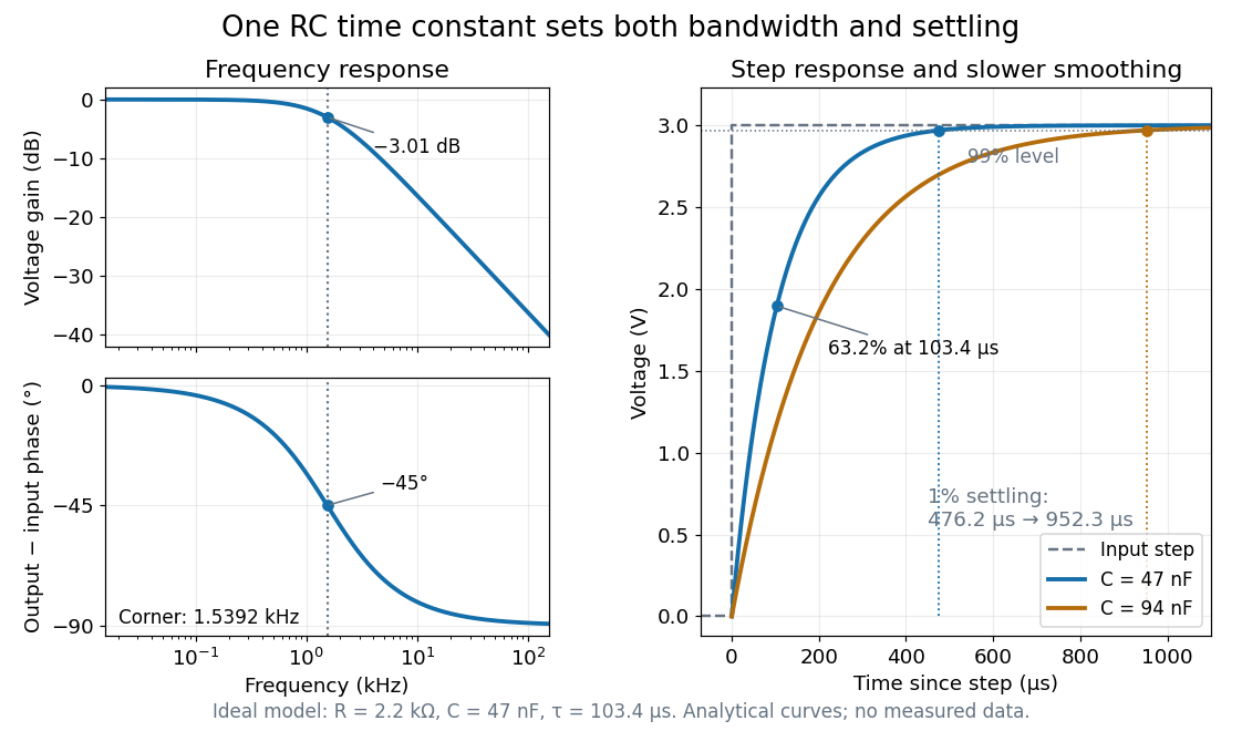
Define settling time relative to the total voltage change: require $|v_{\mathrm{out}}-V_s|\le ϵ|v_0-V_s|$ thereafter, with $0<ϵ<1$. The exponential decay is monotone, soFor $1\%$ settling, $t_{0.01}=4.6052\tau \approx 476.17\mu \mathrm{s}$; the $10\%$ to $90\%$ rise takes $\tau \ln 9\approx 227.19\mu \mathrm{s}$. Reducing the cutoff frequency by doubling $C$ doubles both times. This reciprocal relation is the useful connection between signal bandwidth and response speed: stronger suppression of rapid noise comes with slower tracking of wanted changes.

Use the complex amplitude convention $v(t)=\mathrm{Re}(\hat{V}{e}^{\mathrm{i}\omega t})$, where $\omega =2\pi f$ is the angular frequency and $f$ is the frequency in cycles per second. Substitution into the RC low-pass filter equation replaces the time derivative with multiplication by $\mathrm{i}\omega$, giving its continuous-time frequency responseHere $\varphi$ is the output-minus-input phase difference; a negative value means the output lags. Equivalently, the voltage divider formed from the electrical impedances $R$ and $1/(\mathrm{i}\omega C)$ gives the same ratio. For an input $A\cos (\omega t)$, the sustained output is $A|H|\cos (\omega t+\varphi )$ after the initial exponential decay has died away.

Define the cutoff frequency by a voltage amplitude ratio $1/\sqrt{2}$ relative to the low-frequency value:On a Bode plot, the voltage gain in decibels isAt the cutoff frequency it is $-3.0103\mathrm{dB}$, and far above that frequency it approaches a decrease of $20\mathrm{dB}$ per factor of ten in $f$. There is a smooth transition rather than an abrupt wall. The squared voltage ratio is one half at the corner; converting that statement to a power ratio requires the same real electrical resistance for the compared voltages. It does not mean that an unloaded capacitor dissipates half the source power.

For $R=2.2\mathrm{k}\Omega$ and $C=47\mathrm{nF}$, the cutoff frequency is $f_c\approx 1.5392\mathrm{kHz}$. A $1\mathrm{V}$ peak input at $0.1f_c$, $f_c$, and $10f_c$ produces peak output amplitudes of approximately $0.9950\mathrm{V}$, $0.7071\mathrm{V}$, and $0.09950\mathrm{V}$, with phase differences $-5.711^{\circ }$, $-45^{\circ }$, and $-84.289^{\circ }$. Thus a wanted oscillation at $0.1f_c$ is almost preserved while an unwanted one at $10f_c$ is reduced by about a factor of ten in voltage. The superposition principle lets these two responses be added when both oscillations occur in the same signal.

For axisymmetric inviscid modes between impermeable cylinders in a thin annulus, let $A=2\Omega +r{\Omega }^{\prime }$ and ${\kappa }_{\mathrm{ep}}^2=2\Omega A=r^{-3}(r^4{\Omega }^2{)}^{\prime }$. The linear azimuthal equation gives $u_{\varphi }=-iA{u}_r/\omega$ and the axial equation gives $u_z=k\pi /\omega$, where $\pi$ is the kinematic pressure perturbation. Thin-gap incompressibility implies $\pi =i\omega u_r^{\prime }/k^2$. Eliminating it from the radial equation gives the title equation with $u(R_{<})=u(R_{>})=0$. If a plus sign is used for the potential, its coefficient must be defined as $\Phi =-{\kappa }_{\mathrm{ep}}^2$, the negative of the usual Rayleigh discriminant.

For the Rashba effect with $k_R>0$, put $D=\sqrt{k_R^2+2m{E}_F/{\hslash }^2}$. If $-E_R<E_F<0$, both Fermi contours belong to the lower branch and bound the singly occupied annulus $k_R-D<k<k_R+D$; the central disk and exterior are empty. At $E_F=0$, the lower occupied disk has outer radius $2k_R$, while the origin is a degenerate point at the Fermi energy. For $E_F>0$, the lower Fermi contour has radius $k_{-}=D+k_R$ and the upper Fermi contour radius $k_{+}=D-k_R$. The inner disk has two occupied spin-split eigenstates at each momentum, the intervening annulus has one, and the exterior is empty. Consequently $k_{-}-k_{+}=2k_R$, whereas below the crossing the two lower-branch radii add to $2k_R$. At zero temperature, changing occupation values only on these Fermi contours affects a null set and leaves the integrated carrier density unchanged.

For $H_R=\lambda (k_x{\sigma }_y-k_y{\sigma }_x)$ with $\lambda >0$, the lower- and upper-band spinors of unit norm can be chosen asTheir spin expectation values are $⟨\mathbf{S}{⟩}_{\pm }=\pm (\hslash /2)(-k_y,k_x,0)/k$. They are tangential to circles of constant momentum magnitude, opposite between branches, and reversed at opposite momenta as required by time-reversal symmetry. When $E_F>0$, the outer contour belongs to the lower branch and the inner one to the upper branch. For $E_F<0$ the two Fermi contours both belong to the lower branch and have the same tangential spin orientation at a given angle in polar coordinates. At $k=0$ the Hamiltonian has quantum degeneracy in spin, and no unique spin texture direction is selected.

For the stipulated A/B ideal solution, put $x=x_A$. At the fixed temperature $300\mathrm{K}$, Raoult's law reduces toThe relative volatility is $\alpha =p_A^{\ast }/p_B^{\ast }=4$. For $0<x<1$,Hence every interior vapor-liquid equilibrium pair in this chosen model has A-enriched vapor; neither pure endpoint is enriched. Conversely,For example, $y_A=1/2$ corresponds to $x_A=1/5$, $p_A=p_B=16\mathrm{kPa}$ and $P=32\mathrm{kPa}$. Equal vapor mole fractions therefore need not mean equal liquid mole fractions.

These are fixed-temperature predictions. During boiling at a specified external pressure, the temperature instead adjusts until ${\sum }_i{x}_i{p}_i^{\ast }(T)=P_{\mathrm{external}}$. The two stipulated vapor pressures specify only one temperature; they provide no boiling-temperature curve.

A measurable function $g$ applied to a random variable $X$ defines a new random variable $Y=g(X)$. Its probability distribution is the pushforward measure under $g$.

Raman spectroscopy measures shifted scattering of light to infer internal energy spacings and the molecular response that makes them visible. In a modern illustrative arrangement, narrowband laser illumination replaces the historical arc, an optical filter rejects the strong excitation line, and a spectrograph resolves the weak shifted spectral lines. The illumination, rejection and spectral dispersion are separate jobs. Increasing rejection can conceal small Raman shifts close to the excitation line.

A proposed measurement should record the excitation wavelength, a dark signal, a blank container and the liquid, then compare calibrated line positions and integrated signals under the same collection conditions. Measure optical filter transmission and detector response before using the Thermal Raman line ratio for temperature. Repeat at lower incident power to look for heating or altered sample response. These are suggested checks, not an assertion that the 1928 apparatus implemented modern calibration procedures.

Its appeal is the conversion of internal molecular energy differences into visible spectral lines: changing the excitation can move the whole pattern while preserving characteristic Raman shifts. Combined with vibrational infrared activity, Raman vibrational activity supplies complementary information about molecular vibration. A line pattern can constrain a material's identity or environment, but overlapping bands, fluorescence backgrounds and the finite spectral resolution element prevent an unqualified identification from one peak alone.

Assume one harmonic normal mode at thermal equilibrium, weak spontaneous excitation far from electronic resonances, the same collection solid angle and wave polarization, and matched response after instrumental correction. The Boltzmann distribution givesHere $k_B$ is the Boltzmann constant, $T>0$ is temperature, and $P_v$ is the probability of vibrational quantum number $v$. Thus $P_1/P_0=r$. Linear coupling to $Q$ has squared oscillator matrix elements proportional to $v+1$ for Stokes Raman scattering and $v$ for Anti-Stokes Raman scattering. Summing over initial levels gives strengths proportional to $\overline{v}+1$ and $\overline{v}$ respectively; their ratio is $r$, even when levels above $v=1$ are occupied.

Let $I_{\mathrm{S}}$ and $I_{\mathrm{AS}}$ denote line-integrated radiant intensities, meaning power per collection solid angle. The off-resonant electric dipole radiation law adds the fourth power of emitted frequency:The photon rate divides each line's power by its own $h{\nu }_s$. Consequently, the ideal response-corrected anti-Stokes/Stokes count-rate ratio has the third power of the same frequency ratio. Peak heights alone do not give line-integrated radiant intensities if linewidths differ. Uncorrected detector counts can also include unequal detector response and unequal optical filter transmission. Resonant enhancement, overlapping spectral lines, nonthermal populations and local optical heating can invalidate a temperature inferred from this simple formula.

The simplest off-resonant explanation is a vibrating polarizability. Let $Q(t)=Q_0\cos (2\pi {\nu }_{v}t)$ be a small normal mode coordinate of molecular vibration, and use one scalar component of polarizability, $\alpha (Q)\simeq {\alpha }_0+{\alpha }_0^{\prime }Q$. For incident electric field $E(t)=E_0\cos (2\pi {\nu }_{0}t)$, the induced electric dipole moment isThe product-to-sum formula produces the two displaced frequencies. A nonzero derivative ${\alpha }_0^{\prime }$ gives vibrational Raman scattering in this linear model. Real polarizability is generally a tensor, and the selected components depend on incident and observed wave polarization. This condition differs from vibrational infrared activity, which requires a changing molecular electric dipole moment without an applied optical electric field. A vibration can therefore appear in one measurement and be absent in the other.

This classical modulation argument explains line locations but supplies equal sideband wave amplitudes; it does not explain their thermal asymmetry or the nonzero Stokes Raman scattering from a vibrational ground state. Those require the quantum harmonic oscillator population and transition strengths. The far-off-resonance drawing uses dashed virtual intermediate levels: they represent terms in a scattering probability amplitude, not a long-lived occupied electronic energy eigenstate. Near an electronic resonance, a more detailed treatment of the intermediate response is needed.