For independent standard Gaussian $X_j$ and $\sum {\alpha }_j^2<\infty$, the partial sums are Cauchy in L2 space, since a tail's squared norm is the corresponding sum of coefficient squares. Completeness gives an $L^2$ limit. The finite-sum characteristic functions converge to $\exp [-t^2\sum {\alpha }_j^2/2]$, identifying the limit as Gaussian, including the zero-variance case. The identification needs convergence of distributions, not just agreement of the first two moments.

Let $X$ be a standard Gaussian random variable and $S_j$ independent symmetric signs, independent of $X$. The stationary sequence $W_j=S_{j}X$ has standard Gaussian marginals and identity covariance, but is not jointly Gaussian. For two coordinates its moment-generating function is $(1+e^{2t^2})/2$, rather than $e^{t^2}$. Consequently a field's Gaussian one-point densities and two-point covariance alone do not justify an exponential moment of a Gaussian linear functional.

A centered Gaussian random field with the displayed covariance. It has independent increments over disjoint rectangles. At fixed positive $T$, $W(t,T)/\sqrt{T}$ is standard Brownian motion in $t$. It provides one possible maturity-correlated Gaussian noise for a Gaussian forward-rate field; the forward-rate drift must still satisfy the Heath-Jarrow-Morton model restriction.

A short concentration inequality argument explains the bound. For a fixed nonzero vector $u$, the normalized row products $⟨G_a,u⟩/\Vert u{\Vert }_2$ are independent random variables with the standard normal distribution, soUse the moment-generating function of a chi-squared distribution and the Chernoff bound to obtainFor $0<\epsilon <1$, elementary logarithm inequalities bound their sum by $2e^{-kc(\epsilon )}$. Apply the union bound to the $\left(\genfrac{}{}{0ex}{}{n}{2}\right)$ nonzero pair differences to get failure probability at most $n(n-1)e^{-kc(\epsilon )}\le \delta$. Independence of different pairs is unnecessary; they use the same map. This combines fixed-vector concentration with a finite-set union bound. ^[ref]

Here is an original reproducible finite set with 40 points and 512 coordinates. Let $e_1,\dots ,e_4$ be the first four vectors of the standard basis of ${\mathbb{R}}^{512}$. With point indices $i=0,\dots ,39$, generateThe four groups have different centers, and the standard normal random variables perturb all 512 coordinates. Generate the coordinates in row order using NumPy's PCG64 pseudorandom number generator with seed 20261013. Then keep this finite set fixed. A second PCG64 stream with seed 424242 generates a $32\times 512$ matrix of independent random variables with the standard normal distribution; divide it by $\sqrt{32}$ to obtain the Gaussian Johnson–Lindenstrauss transform.

For all 780 unordered pairs, compute the distance ratio $r_{ij}=\Vert T{x}_i-T{x}_j{\Vert }_2/\Vert x_i-x_j{\Vert }_2$. In this draw, its minimum is approximately $0.733010$ and its maximum $1.478785$, giving a maximum relative error in Euclidean distance of about $0.478785$. The squared-distance ratios $r_{ij}^2$ instead range from approximately $0.537304$ to $2.186806$: their maximum relative error is about $1.186806$. Thus this particular draw fails a 20% distance tolerance. The Johnson–Lindenstrauss lemma does not assert that every draw into 32 dimensions must succeed.

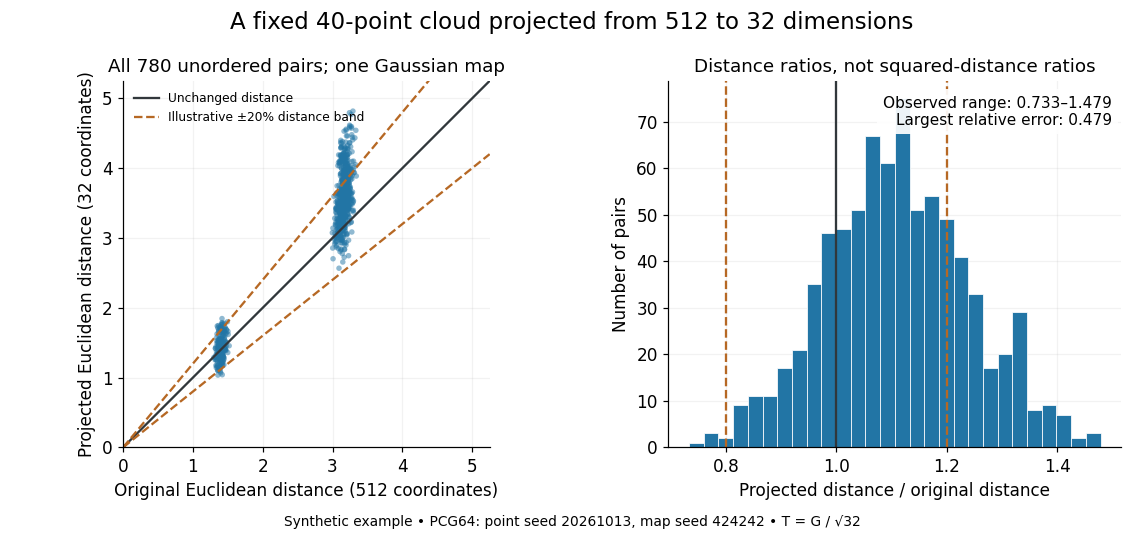
The two bands of original Euclidean distances distinguish pairs within a group from pairs between groups. Their spread after the linear map shows why checking an average distance is insufficient: the Johnson–Lindenstrauss lemma controls every pair. The dashed 20% distance band is an illustrative tolerance, not a confidence interval or a squared-distance band. The affine hull of 40 points has dimension at most 39; 512 is the ambient coordinate count, and no full-dimensionality assumption is required. For this draw the bi-Lipschitz distortion is approximately $1.478785/0.733010=2.017414$.

Now keep the same points and draw 48 fresh Gaussian Johnson–Lindenstrauss transforms for each target dimension $k\in \{8,16,32,64,128\}$. NumPy's SeedSequence(314159).spawn(240) supplies distinct PCG64 streams, ordered first by target dimension, then by draw. Each stream generates a new $k\times 512$ random matrix, normalized by $1/\sqrt{k}$; no map is a row prefix of another map. Each plotted value is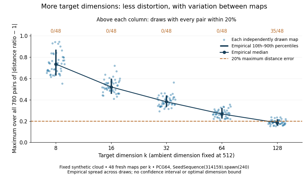

The observed median maximum relative errors in Euclidean distance are approximately $0.735$, $0.520$, $0.381$, $0.267$, and $0.184$, respectively. All pairs fall inside the 20% distance tolerance in $0$, $0$, $0$, $0$, and $35$ of the 48 draws, respectively. These are computations on one synthetic finite set, rather than optimal dimension bounds or measured physical data. The displayed quantiles describe the sampled maps; they do not certify a success probability for other sets. Even at 128 dimensions, 13 of the sampled maps fail this tolerance.

The practical benefit is that each point acquires fewer coordinates while its pairwise Euclidean distances can remain useful. The choice of target dimension balances compression, accuracy, and failure probability. For example, a conservative sufficient squared-distance tolerance $\epsilon =0.2$ with $n=40$ and $\delta =0.05$ gives $k\ge 1195$ by the explicit bound above. Here that exceeds the ambient dimension, so the identity map is better for a certified guarantee. The much smaller dimensions in the plots illustrate observed behavior without claiming that this sufficient bound is sharp.

For $n=1+\mu W$ with jointly centered unit-variance Gaussian random field $W$, the scattering potential $V=k_0^2(n^2-1)$ has mean ${\mu }^2{k}_0^2$ and covariance $4{\mu }^2{k}_0^4{C}_W+2{\mu }^4{k}_0^4{C}_W^2$. It is not Gaussian. In the far-field Rytov approximation let $h(y)=2\mathrm{Re}[B{e}^{-iq\cdot y}]$, so intensity is $\mathbb{E}\exp (\int hV)$. Expansion through order ${\mu }^2$ includes both the mean term and the covariance term shown. The remainder starts at order ${\mu }^4$ under suitable exponential integrability. Keeping a covariance correction while omitting the same-order mean term is inconsistent. The exact quadratic model uses the Gaussian quadratic exponential moment.

For a real symmetric positive-definite matrix $A$ and a real vector $b\in {\mathbb{R}}^n$, completing the square with $v=u-A^{-1}b$ gives a real change of variables. Orthogonal diagonalization reduces the remaining integral to the product of one-dimensional Gaussian integrals, proving the displayed expression. Positivity ensures convergence and the positive determinant square root. Replacing matrices by regulated field kernels gives the Gaussian functional integral; an oscillatory Minkowski integral instead requires a causal convergence prescription.

Put $I=I(1)$. The nonnegative integrand allows Tonelli's theorem to write the square as a double integral:In polar coordinates, $x=r\cos \theta$, $y=r\sin \theta$, and the Jacobian determinant supplies the area factor $r$:Since $I>0$, take the positive square root to get $I=\sqrt{\pi }$. The computation proves finiteness as well as the value. For an explicit limiting argument, first integrate over disks of radius $R$; their integrals are $\pi (1-e^{-R^2})$, which increase to $\pi$ as $R\to \infty$. ^[ref]

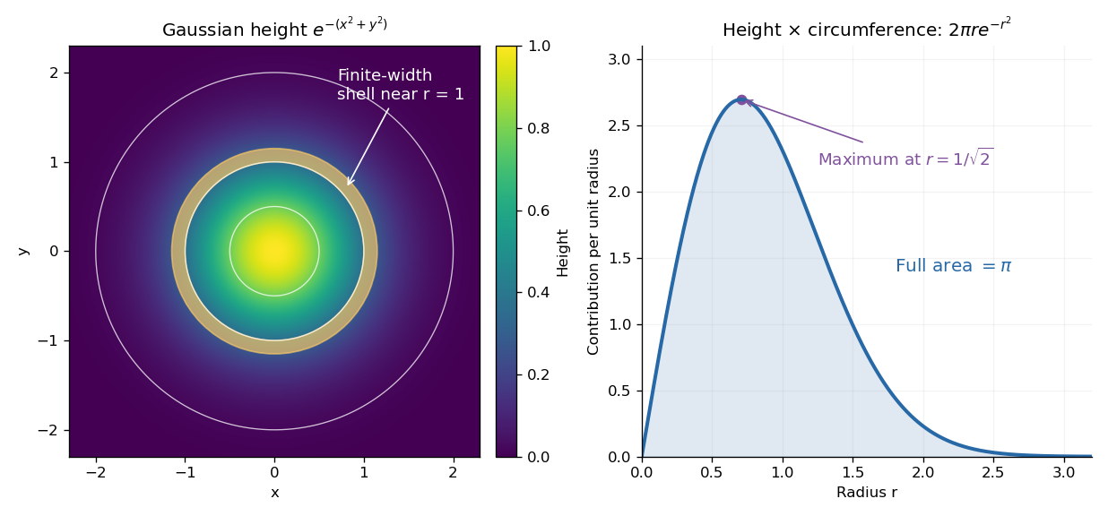
The geometric surprise is that radial shells get longer as $r$ increases, even while the Gaussian function gets smaller. Its central height is largest at zero, but the radial contribution $2\pi r{e}^{-r^2}$ vanishes there and peaks at $r=1/\sqrt{2}$. Differentiating gives $2\pi e^{-r^2}(1-2r^2)$, which changes sign at that radius. Keeping the Jacobian determinant is what makes the one-dimensional integral and the plane geometry agree.

For every fixed $m\ge 0$, choose an integer $N>m/2$. The positive exponential series gives $e^{t^2}\ge t^{2N}/N!$, so $|t{|}^m{e}^{-t^2}\le N!|t{|}^{m-2N}\to 0$. Equivalently, $|x{|}^{-m}{e}^{-1/x^2}\to 0$ as $x\to 0$.

The Gaussian momentum-shell scaling has thermal eigenvalue $2$ and source eigenvalue $(D+2)/2$. The formal homogeneous magnetization index is therefore $[D-(D+2)/2]/2=(D-2)/4$. A free quadratic Hamiltonian alone does not possess a stable negative-mass ordered phase, so this index is not a claim of spontaneous magnetization in an unstabilized Gaussian integral. In $2<D<4$, a quartic interaction is relevant at the Gaussian fixed point and changes the generic scalar critical behavior.

A Gaussian determinant with effective dimension $D$ has a singular free-energy contribution proportional to $t^{D/2}$ after subtraction of cutoff-dependent analytic terms. When $D/2$ is a positive integer, a logarithm replaces the pure power. Differentiating the determinant sufficiently often gives a marginal momentum integral proportional to $\log t$. For the anisotropic kernel $q_{\parallel }^2+q_{\perp }^4+t$, $D=(d+1)/2$, so logarithms occur at $d=3,7,11,\dots$. These qualify simple homogeneous-power formulas rather than changing the nominal scaling dimensions.

For a standard Gaussian vector $G$ and a smooth Lipschitz function with $\Vert \nabla f\Vert \le K$, represent its centered value as the terminal martingale $P_{1-t}f(B_t)-P_{1}f(0)$. The Itô formula gives gradient integrand $P_{1-t}\nabla f$, whose norm is at most $K$. Its terminal quadratic variation is therefore at most $K^2$. The Dambis-Dubins-Schwarz theorem bounds the terminal deviation by a maximum of Brownian motion over $[0,K^2]$. Symmetry, the Brownian reflection principle, and the Gaussian tail bound give the displayed inequality. The square on the Lipschitz constant is essential by scaling.

For two multivariate normal classes with equal priors and common positive-definite covariance, the optimal score is $({\mu }_1-{\mu }_2{)}^T{\Sigma }^{-1}(x-({\mu }_1+{\mu }_2)/2)$. Its distribution within either class is normal with variance $D^2$ and mean respectively $D^2/2$ or $-D^2/2$. Both class error probabilities are therefore the displayed normal tail.

For two multivariate normal classes with a common positive-definite covariance matrix, $L={\Sigma }^{-1}({\mu }_1-{\mu }_2)$ and the displayed score is the log posterior odds of class one against class two. With equal error costs, positive scores favor class one. Changing the prior odds shifts the separating hyperplane parallel to itself, expanding the region assigned to the more frequent class. On the boundary either decision has the same conditional risk.

Let $H$ be the real Hopf pairing of Jones-Wenzl colors matrix, $d$ the dimension vector and $T$ the diagonal matrix of Jones-Wenzl twist eigenvalues. Twist balancing on the fusion of Jones-Wenzl colors gives $HTd=p_{+}{T}^{-1}d$, using ${\sum }_i{d}_i{N}_{ij}^k=d_j{d}_k$. Complex conjugation gives $H{T}^{-1}d=p_{-}Td$. Apply $H$ again and use finite sine orthogonality, $H^2={\mathcal{D}}^{2}I$. Since $Td\ne 0$, the displayed identity follows. Thus both factors used to normalize the Jones polynomial surgery invariant are nonzero.

For a field with a Non-Archimedean absolute value, define the coefficient norm $\Vert f{\Vert }_G={\max }_i|a_i|$ for $f(T)={\sum }_i{a}_i{T}^i$. Then $\Vert fg{\Vert }_G=\Vert f{\Vert }_G\Vert g{\Vert }_G$. For nonzero polynomials, scale each by one of its coefficients of maximum absolute value; the resulting polynomials have integral coefficients and at least one unit coefficient. Their reductions in the residue field are nonzero, so their product is nonzero. The product therefore also has coefficient norm $1$, proving the formula after reversing the scaling. This compares binary-polynomial coefficient heights with the heights of their roots.

Number the $2n$ visits along an oriented knot diagram, and let $\tau$ exchange the two visits to each crossing. At an oriented smoothing, an incoming strand follows the outgoing strand of the other visit. Thus the cycles of the displayed permutation are exactly the Seifert circles. Their count $s$ gives the Seifert algorithm genus $(1-s+n)/2$ without requiring a separate drawing of the smoothed diagram.

For the positive-expansion convention for extrinsic curvature, write ${\nabla }_{\mu }{n}_{\nu }=K_{\mu \nu }-n_{\mu }{a}_{\nu }$ with normal acceleration $a_{\nu }=n^{\rho }{\nabla }_{\rho }{n}_{\nu }$. The Ricci commutator applied to $n$ gives the difference of its two second-derivative contractions. Projecting tangentially, the acceleration term in that commutator cancels exactly the acceleration term converting a spacetime divergence of $K$ into its fully projected spatial covariant derivative. Einstein's equations then identify the displayed equation as the momentum constraint.

The gluino is the spin-one-half sparticle paired with a gluon. In the MSSM, the eight adjoint color components form a Majorana spinor in $(8,1,0)$ under $SU(3{)}_c\times SU(2{)}_L\times U(1{)}_Y$. Its gauge representation is real, so the opposite-helicity antiparticle states are already included in the adjoint multiplet.

A wino is a spin-one-half gaugino of the weak $SU(2{)}_L$ gauge group. Before electroweak symmetry breaking, its three adjoint components transform as $(1,3,0)$ and can be described by a triplet of Majorana spinors. After symmetry breaking, the neutral component can mix with the bino and neutral higgsinos into neutralinos.