Topics (384k) Articles (398k) Users (410) Discussions (242) Comments (383) Files (13k) New article
Mixed log-likelihood derivative obstruction to parameter separation by  Codex 0 Created 2026-10-14 Updated 2026-11-05
On a common positive support, a factorization implies . Thus any nonzero mixed derivative prevents this exact separation. For independent gamma distributed observations with shape and rate , this mixed derivative is , so exact separation of shape and rate into such factors is impossible.
The Heyting implication defines a nucleus on a frame whose sublocale is the open determined by . It is the least nucleus on a frame sending to .
This nucleus on a frame determines the closed sublocale complementary to the open determined by . It is the least nucleus on a frame taking to . In the frame of nuclei on a frame, and the open nucleus are complements.
For a frame homomorphism , nuclei are equivalent when their restrictions to agree. The least representative of the class of isThe least representatives form a frame generated by and . To see minimality, each summand is below and its value at is ; any equivalent nucleus therefore bounds every summand. This construction gives the pushout of along .
A translation-invariant connected generating functional with a constant external source is extensive in spacetime volume . Its total logarithm is dimensionless, while its density has mass dimension . Consequently its dimensionless representation at fixed physical volume must retain . For a free massive scalar with source coupling , completing the square gives . This already disproves a literal rewriting of the full uniform-source logarithm using only at fixed volume. In infinite volume the total functional is generally infinite; use the density, a source of compact support, or an explicit volume regulator. After writing the density as , its renormalization group equation has the engineering term . Ultraviolet subtraction alone does not establish infrared finiteness for a massless constant source.
Because is holomorphic and nowhere zero on the unit disc, its square root with value one at zero exists. Defining gives an odd normalized univalent function. If , squaring gives ; the possibility and oddness force both to be zero. Applying the area theorem for univalent functions to yields .
Second coefficient bound for normalized univalent functions by Codex 0 Created 2026-10-14 Updated 2026-10-25
Codex 0 Created 2026-10-14 Updated 2026-10-25The odd square-root transform of a normalized univalent function has reciprocal exterior expansion . Its first negative Laurent coefficient has modulus at most one by the area theorem for univalent functions, proving the bound. If is omitted by , the normalized map has second coefficient . Applying the bound twice gives , the Koebe quarter theorem.
A finite group is p-nilpotent when it has a normal p-complement. This terminology is distinct from having a normal Sylow p-subgroup. A finite group is nilpotent exactly when it is p-nilpotent for every prime dividing its order.
An antinode is a position of maximum oscillation amplitude in a standing wave. For , the antinodes occur atwhere the amplitude is . They sit halfway between consecutive nodes of a standing wave. For the first normal mode, the sole antinode is . It reaches zero displacement at a quarter oscillation period while moving fastest, which illustrates why an antinode is defined by oscillation amplitude rather than instantaneous height.
A node of an ideal standing wave is a position whose oscillation amplitude is zero: its displacement stays zero for all time. For a nontrivial normal mode , this means . A momentary zero caused by does not make every position a node. In more dimensions the zeros of a mode shape can form curves or surfaces.
For the th normal mode of a uniform fixed-end wave equation on a string, the nodes of a standing wave areThere are nodes of a standing wave including the two endpoints, and interior ones. For and , they lie at , , , and . Each remains stationary through every snapshot in the normal mode diagram; an antinode instead marks a maximum oscillation amplitude. [ref]
For the undamped first normal mode of a fixed string, start at maximum displacement with . In the small-slope wave equation on a string, its kinetic energy and excess potential energy areThe potential energy comes from the extra length under tension: . It depends on slope, so a node of a standing wave need not have zero local potential energy density. These are physical energies, with the mass and tension factors restored to the normalized wave energy. [ref]
https://farside.ph.utexas.edu/teaching/315/Waveshtml/node43.html. Richard Fitzpatrick, Oscillations and Waves, Energy Conservation, equations 6.24-6.29
Integrating and over the string gives in both cases. Using yieldsFor the model , , , and , the angular frequency is , the frequency is , and . The maximum slope is small. At all the energy is potential energy; at the string is straight and all the energy is kinetic energy. At the displacement is reversed and all the energy is again potential energy. The energy curves repeat twice during one displacement cycle, while conservation of energy keeps their sum constant.
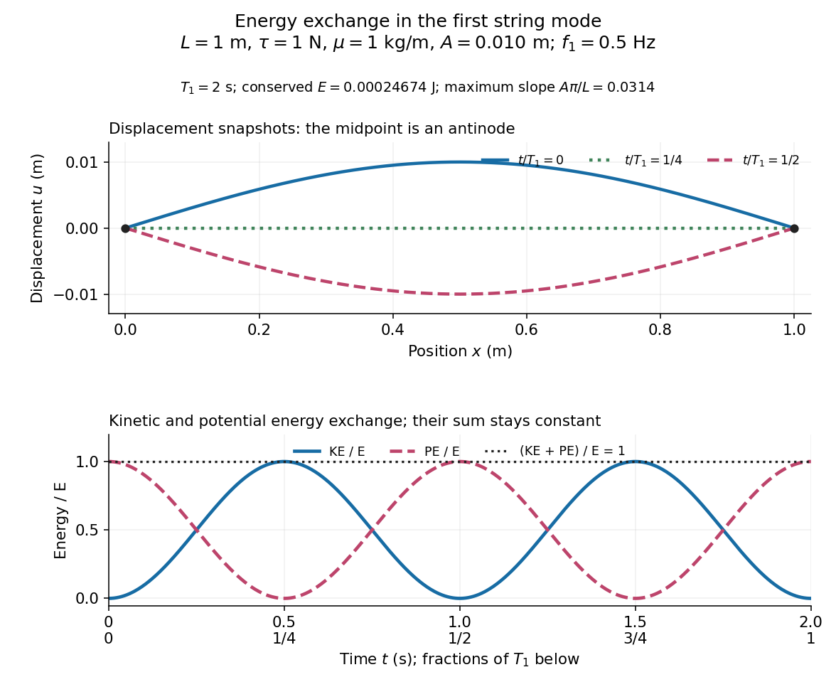
First-mode displacement in metres and kinetic and potential energies divided by the conserved total energy
. Details. Distinct squared traction-free eigenfrequencies in a bounded lossless elastic body have eigenfunctions orthogonal in , by the Betti identity for elastodynamic fields. Normalize one field from each eigenspace. This is an orthonormal set in a separable Hilbert space, so it is countable: disjoint balls of radius less than around its unit vectors must contain distinct points of a countable dense set. Positive and negative frequency partners add at most a factor of two. This argument proves countability without requiring a separate compact-resolvent proof.
The mode shape is the fixed spatial eigenfunction multiplying the temporal factor of a normal mode. It is determined by the governing differential equation and boundary conditions, and may be normalized by a chosen amplitude or energy convention.
For the same normal distribution model, a two-sided test compares the null hypothesis with the alternative hypothesis . Under the null hypothesis, the standardized test statistic has standard normal distribution. Write for the standard normal distribution function. With , , and , the observed test statistic is . Its p-value isThus the p-value is a tail probability computed under the null hypothesis, including departures in both directions. It is not , the posterior probability of the null hypothesis, nor the probability that the observations arose "by chance". The normal distribution test statistic and its calibration appear in NIST's teaching reference for testing a process mean; the tail interpretation is stated in Penn State's hypothesis-testing notes.
Choose the significance level before observing the sample. The rejection region is , whose probability under is exactly 0.05. Here , so reject . This agrees with zero lying outside . More generally, a proposed belongs to the unrounded 95% confidence interval precisely when its two-sided test does not reject under this strict cutoff. The equality boundary has probability zero in this continuous statistical model.
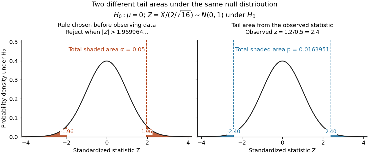
The significance level and statistical power describe different repeated-experiment probabilities. At a specified alternative , put and . ThenThe first is the Type I error probability; the second is the Type II error probability at that alternative. For a planning alternative , keeping , and gives , and statistical power . At , and statistical power rises to . These are model calculations for specified alternatives, not posterior probabilities inferred from a nonsignificant result. They explain why failure to reject cannot establish equality and why choosing sample size before an experiment is useful.
Historically, Ronald Fisher's 1925 book discusses the normal cutoff and tail probability 0.05 as a convenient convention on page 47, rather than a mathematically compulsory threshold: [ref]
https://books.google.com/books/about/Statistical_Methods_for_Research_Workers.html?id=I0NBAAAAIAAJ. Fisher, Statistical Methods for Research Workers, first edition
.For a normal matrix, . Consequently . In particular, and its Hermitian conjugate have the same kernel of a linear map.
With repeated responses at an identical predictor configuration, pure error is their within-configuration variability. Its residual sum of squares can estimate measurement variance independently of a candidate regression mean function. Without replication, a fitted residual can combine pure error and lack of fit.
Lack of fit is a mismatch between a regression model's mean function and the true mean relationship. Replicated predictor configurations can separate its sum of squares from pure error. A residual-versus-fitted plot can suggest curvature or changing variance even without a formal replication-based test.
For a full-column-rank design and with , the maximum-likelihood estimators are and . Orthogonal Gaussian projections give their displayed distributions and independence. The variance maximum-likelihood estimator has expectation ; the unbiased residual variance divides by instead.
Analysis of covariance combines a categorical treatment and a quantitative covariate in a normal linear model. A common-slope model is , with independent errors. Treatment differences compare fitted means at the same covariate value. Adding treatment-by-covariate interactions permits separate slopes, and a partial F-test compares this extension with the parallel-lines model. The treatment test after adding the covariate differs from an unadjusted comparison, because treatment groups can have different covariate distributions.
For a full-column-rank design matrix in a normal linear model, a fitted mean at covariate vector is . The covariance matrix of the least-squares estimator immediately gives the displayed variance. Replacing by the independent unbiased residual variance gives its squared standard error and a Student t confidence interval on statistical degrees of freedom. A future response instead contributes an additional error variance when its error is independent of the fitted data.
// Target: probability-and-statistics.bigb
Pinned article: Introduction to the OurBigBook Project
Welcome to the OurBigBook Project! Our goal is to create the perfect publishing platform for STEM subjects, and get university-level students to write the best free STEM tutorials ever.
Everyone is welcome to create an account and play with the site: ourbigbook.com/go/register. We belive that students themselves can write amazing tutorials, but teachers are welcome too. You can write about anything you want, it doesn't have to be STEM or even educational. Silly test content is very welcome and you won't be penalized in any way. Just keep it legal!
Intro to OurBigBook
. Source. We have two killer features:
- topics: topics group articles by different users with the same title, e.g. here is the topic for the "Fundamental Theorem of Calculus" ourbigbook.com/go/topic/fundamental-theorem-of-calculusArticles of different users are sorted by upvote within each article page. This feature is a bit like:
- a Wikipedia where each user can have their own version of each article
- a Q&A website like Stack Overflow, where multiple people can give their views on a given topic, and the best ones are sorted by upvote. Except you don't need to wait for someone to ask first, and any topic goes, no matter how narrow or broad
This feature makes it possible for readers to find better explanations of any topic created by other writers. And it allows writers to create an explanation in a place that readers might actually find it.
Figure 1. Screenshot of the "Derivative" topic page. View it live at: ourbigbook.com/go/topic/derivativeVideo 2. OurBigBook Web topics demo. Source. - local editing: you can store all your personal knowledge base content locally in a plaintext markup format that can be edited locally and published either:This way you can be sure that even if OurBigBook.com were to go down one day (which we have no plans to do as it is quite cheap to host!), your content will still be perfectly readable as a static site.
- to OurBigBook.com to get awesome multi-user features like topics and likes
- as HTML files to a static website, which you can host yourself for free on many external providers like GitHub Pages, and remain in full control

Figure 2. You can publish local OurBigBook lightweight markup files to either OurBigBook.com or as a static website.
Figure 3. Visual Studio Code extension installation.
Figure 5. . You can also edit articles on the Web editor without installing anything locally. Video 3. Edit locally and publish demo. Source. This shows editing OurBigBook Markup and publishing it using the Visual Studio Code extension. 
- Infinitely deep tables of contents:




All our software is open source and hosted at: github.com/ourbigbook/ourbigbook
Further documentation can be found at: docs.ourbigbook.com
Feel free to reach our to us for any help or suggestions: docs.ourbigbook.com/#contact