Topics (384k) Articles (398k) Users (410) Discussions (242) Comments (383) Files (13k) New article
A second-order reaction has overall order of reaction two: a rate law may depend on , or on with partial orders of reaction one and one. Doubling all relevant reactant concentrations multiplies the reaction rate by four at fixed conditions. This experimentally determined dependence does not establish molecularity or a unique reaction mechanism. For an elementary reaction obeying the law of mass action, molecularity and overall order of reaction agree; a net chemical equation alone cannot establish that the conversion is elementary.[ref]
Glossary of Terms Used in Physical Organic Chemistry (IUPAC Recommendations 1994): N and O entries by International Union of Pure and Applied Chemistry. Glossary of Terms Used in Physical Organic Chemistry, IUPAC Recommendations 1994, entry “order of reaction”, final paragraphs: elementary versus stepwise reactions
For the single-concentration model, explicitly choose the disappearance rate conventionHere is the coefficient for loss of A, held fixed at the specified temperature and other conditions. Its subscript labels the chosen observed disappearance rate; it does not imply a pseudo-first-order reaction. Assume a uniformly mixed closed system, fixed volume, and no appreciable reverse or competing chemical reactions. The integrated rate law isThe reciprocal-concentration plot is a straight line with slope and intercept . A brief derivation uses the chain rule: , then applies the initial condition. This is a hyperbolic decay, rather than the exponential decay of a first-order reaction.[ref]
Chemistry 2e. §12.4, “Second-Order Reactions”, integrated equation and straight-line form; Table 12.2
As an original prescribed example, choose and . At , the reciprocal-concentration calculation is , giving . The initial disappearance rate is ; after it is . Halving the concentration quarters the disappearance rate.
Dimensional analysis checks every formula: has units , has units , and is a dimensionless quantity. Changing concentration units changes the numerical rate constant: the same example is , , giving .
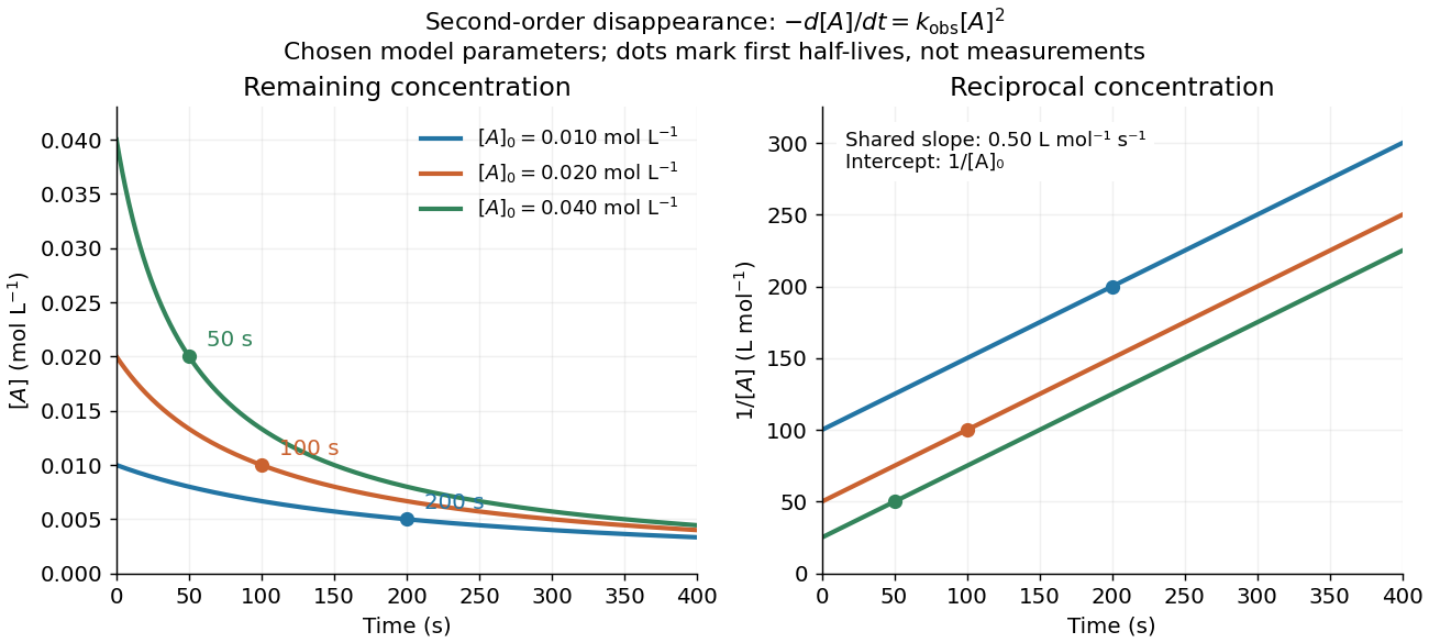
Second-order reaction concentration decay and reciprocal-concentration lines for three prescribed starting concentrations
. Original model curves, not measured data. All use the disappearance rate coefficient . The reciprocal lines share a slope while their intercepts differ; marked points give each run's first half-life. Details.For an elementary reaction , instead define the stoichiometrically normalized reaction rate . Two A entities disappear per P formed, soConsequently the reciprocal-concentration slope is , not . In the prescribed example, the normalized rate constant would be ; initially while the disappearance rate is twice that. With , stoichiometry gives . Both rate constants have the same dimensions, so a units check alone cannot catch their factor-of-two difference. The symbol denotes the same normalization as in reaction rate.
The half-life, meaning the time to reach half a specified starting concentration, follows by setting :For in , this becomes . Its units are seconds because has units . Doubling the starting concentration halves the first half-life; a quoted half-life needs its starting concentration. This differs from a first-order reaction, whose half-life is independent of starting concentration.[ref]
Within the prescribed run, reaches , , and at , , and . The successive halving intervals are , , and : each begins at a smaller concentration. More generally, reaching fraction of the initial concentration, with , requires , so consumption takes nine initial half-lives, rather than a fixed sequence of equal waiting times.
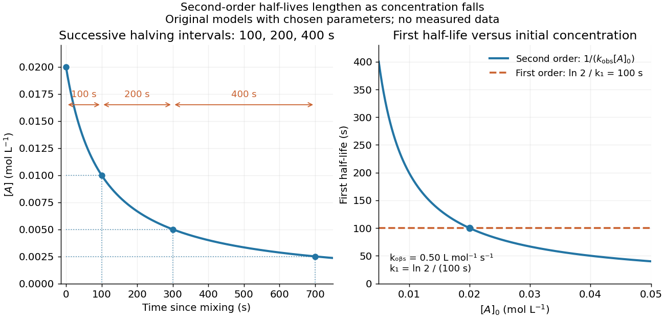
Lengthening second-order reaction halving intervals and the dependence of the first half-life on initial concentration
. Original model predictions, not measurements. Left: the prescribed run. Right: at fixed , compared with a first-order reaction chosen to have . That comparison uses , with different units from . Details.A straight reciprocal-concentration plot tests this particular single-concentration rate equation. It does not uniquely identify a reaction mechanism, nor does curvature rule out every second-order reaction: two independently changing reactant concentrations require their own integrated rate law. At low concentration, a small measurement error becomes approximately in the reciprocal, magnifying late-time errors. Use the line as a diagnostic; a nonlinear regression of the original concentrations can retain their measurement scale and explicit error model.
A zero-order reaction has a reaction rate independent of the relevant reactant concentration over the range where its rate law applies. For , is valid only before depletion at . The constant-consumption model must stop or change there.
A first-order reaction has a reaction rate proportional to one reactant concentration in the simple single-species case. For an irreversible in a closed system at fixed volume, take , , and constant rate constant . Its rate equation and solution areA short check is enough: differentiating gives , and the two concentrations sum to , as required by the one-to-one stoichiometry. Thus the same exponential decay describes both remaining reactant and decreasing reaction rate. Fixed means a fixed fractional loss per unit time, not a fixed absolute consumption rate.
Choose illustrative values and , with measured in seconds. Then , , and . The half-life isAt each successive half-life, half the remaining reactant is consumed; is independent of for this first-order reaction. At , the calculated values are , , and . These are model predictions for chosen parameters, rather than experimental measurements.
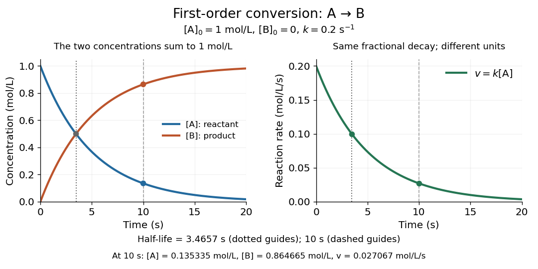
Illustrative first-order reaction: reactant loss, reaction product formation, and declining reaction rate for
. Details. The left panel tracks the two concentrations; the right tracks their instantaneous conversion reaction rate. Their different vertical units matter: , so the numerical curves need not have the same height. This gives a practical way to translate a measured concentration into a forecast of both conversion and waiting time.
A nonzero holomorphic function on the unit disc can have exactly a prescribed sequence of zeros, counted with multiplicity, if and only if that sequence is locally finite in the disc. Necessity is the identity theorem for holomorphic functions. For sufficiency, remove a finite number of zeros at zero and enumerate the others as , so . Use the Weierstrass elementary factors . On every compact subdisc, eventually and . Hence converges locally uniformly and has exactly the prescribed zeros. Finite sequences simply give finite products.
True longitude is the conventional orbital angle formed from the longitude of ascending node, argument of periapsis and true anomaly. For a coplanar Kepler orbit it is the actual polar longitude of the position vector. For an inclined orbital plane the sum of angles is generally not the projected azimuth. The mean longitude uses mean anomaly in place of , so . For small orbital eccentricity, Kepler's equation gives , while the eccentric-to-true anomaly relation gives ; hence . This periodic difference matters when separating a slow resonant argument from a rapidly varying geometric angle.
The argument of periapsis is the angle in the orbital plane from the ascending node to periapsis, measured in the direction of motion. It differs from the longitude of periapsis . For an inclined orbit this sum is a conventional longitude, not generally the azimuth of the projected periapsis. The argument is undefined for a circular orbit and the node-based description is singular when the orbit and reference plane coincide.
The diagonal group action of the symmetric group on ordered pairs has two orbits of a group action when : equal pairs, of size , and distinct pairs, of size . Equality is preserved by a bijection, and a prescribed bijection on one or two distinct letters extends to a permutation of all letters. At only the equal-pair orbit remains.
Call delta equation for a driftless local volatility diffusion by  Codex 0 Created 2026-10-14 Updated 2026-11-05
In the cash-numéraire market , let a smooth call value solve . Its delta hedge is . Differentiating the pricing equation giveswith this terminal condition interpreted away from . If the terminal law has no atom at , its assigned value at that point does not affect expectation pricing; a degenerate or absorbed diffusion can instead require a separate strike-boundary analysis. By Itô formula, , while . Thus holding shares and cash replicates the terminal call. The drift in the option delta equation comes from differentiating the spatially varying diffusion coefficient, not from a drift in the original stock.
For an equiprobable source, an optimal binary prefix tree has leaf depths differing by at most one. If one leaf has depth and a deepest sibling pair has depth , split the shallow leaf into two children and collapse the deep pair into its parent. The number of leaves is unchanged and their total depth decreases by , contradicting optimality.
// Target: probability-and-statistics.bigb
The number of edges on the graph path from the root of a tree to the leaf for symbol in a code tree. The root of a tree has depth zero. Each edge contributes one bit to a binary codeword, so this depth equals the codeword length; weighting these depths by probabilities gives expected codeword length.
For isotropic emission without significant absorption, integrating the spontaneous photon-production rate along the sightline gives the displayed energy intensity per solid angle. Photon intensity omits the factor . Summing unresolved transitions is necessary before comparing with an observed blended spectral feature.
The group refractive index is for a transparent isotropic propagation branch with forward group velocity . Differentiating the local wavenumber givesThe last formula gives the propagation group delay along a path whose geometry is fixed as frequency varies; additional apparatus wave phases require their own frequency derivatives. For a narrow wave packet with little loss and negligible reshaping, it approximates the transit of its wave envelope. In the nondispersive case , it reduces to . An optical path length at one frequency contains no information about , so in a medium with optical dispersion it cannot by itself determine the group delay. [ref]
For an original local model near , choose two equal geometric paths of length , with and . At both optical path lengths equal , and matched launch and interface references give equal carrier wave phases. But and , so their group delays differ by . This local stipulated model is a counterexample to identifying equal wave phase with equal pulse arrival; it asserts no material response outside the narrow band considered. Strong loss or pulse reshaping requires a fuller propagation model, and group delay need not time the earliest causal response.
An optical path difference subtracts two optical path lengths at the same frequency and with specified endpoints and sign. Its phase difference contribution is , in addition to any apparatus reference wave phase. For wavefront error, the comparison is usually between an actual wavefront and an ideal reference wavefront.
For a parallel-transported screen and affine null geodesic tangent , the optical matrix satisfiesIts trace gives the null Raychaudhuri equation. In a two-dimensional screen, symmetric trace-free matrices have scalar squares and anticommute with antisymmetric matrices. The trace-free symmetric and antisymmetric parts consequently yield the null shear and twist transport equations without additional quadratic trace-free terms.
Suppose an extended source fills every position of the entrance aperture with a cone of half-angle , and all these light rays must reach a one-sided planar receiver. If the receiver accepts at most a cone of half-angle , its available etendue bounds the admitted etendue:ConsequentlyThis original derivation combines conservation of etendue with the exact cone integral; the second inequality allows the complete output hemisphere. It bounds capacity and does not prove that a chosen shape attains the bound.
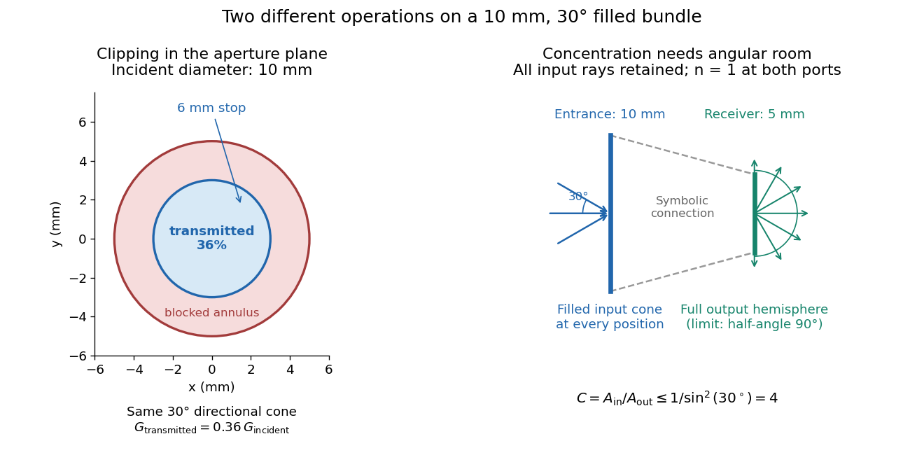
For the input cone with , : a entrance cannot deliver the entire filled bundle to a circular receiver smaller than in diameter. If the output half-angle is restricted to , and the receiver diameter must be at least . For a receiver medium with model refractive index , the full-hemisphere capacity bound instead gives ; that larger value also depends on transmitting the bundle into that medium.
Attempting in the air-to-air example forces rejection of some input. For the uniform radiance already specified, even filling the entire output hemisphere givesThe maximum mean irradiance gain remains . With nonuniform radiance, rejecting a given fraction of geometric etendue need not reject the same fraction of radiant flux.
These bounds use a filled extended-source bundle in passive reversible geometrical optics, comparing the same wavelength and the same radiation channels. An ideal optical point source does not fill that four-dimensional set. Diffraction, optical coherence, or coupling a Gaussian beam into an optical fiber require a physical optics calculation; the cone bound is not a universal guarantee for a single wave mode. Likewise, optical gain or fluorescence changes the propagation assumptions.
For a linear operator bounded from to with norms , , interpolate reciprocals by and . The intermediate operator norm is at most . The complex interpolation proof first treats simple functions; completeness and continuity on the endpoint sum spaces identify the extension with the original operator. On finite counting spaces it also gives norm bounds between sequence spaces.
An open normal subgroup of a topological group is simultaneously open in its topology and invariant under conjugation. For a profinite group, the quotient is a finite discrete group: its cosets form a disjoint open cover, so compactness gives finitely many. Conversely the group homomorphism kernel of a continuous homomorphism to a finite discrete group is open and normal. Such subgroups form an identity-neighbourhood basis of every profinite group.
The Dedekind eta function modular transformation gives . The saddle-point approximation for coefficient extraction has , phase and curvature . Its prefactor supplies and the Gaussian width supplies . This explains both the exponential growth and the power .
Integer-mode expansion with parallel D-brane endpoints by Codex 0 Created 2026-10-14 Updated 2026-11-05
Codex 0 Created 2026-10-14 Updated 2026-11-05On , a coordinate with Neumann boundary conditions at both ends has a constant position, linear time zero mode and cosine oscillators. A coordinate with Dirichlet boundary conditions at both ends has a linear spatial interpolation between endpoint positions and sine oscillators, with no momentum zero mode. Both have integer frequencies. This differs from an ND boundary condition, which applies different conditions at the two ends of the same coordinate and gives half-integer frequencies.
An affine open cover of a scheme is an open cover by affine open subsets. Every scheme has such a cover by definition. A quasi-compact scheme has a finite affine open cover. Whether the intersections are affine is a further condition, supplied in particular by separatedness over an affine base.
Pinned article: Introduction to the OurBigBook Project
Welcome to the OurBigBook Project! Our goal is to create the perfect publishing platform for STEM subjects, and get university-level students to write the best free STEM tutorials ever.
Everyone is welcome to create an account and play with the site: ourbigbook.com/go/register. We belive that students themselves can write amazing tutorials, but teachers are welcome too. You can write about anything you want, it doesn't have to be STEM or even educational. Silly test content is very welcome and you won't be penalized in any way. Just keep it legal!
Intro to OurBigBook
. Source. We have two killer features:
- topics: topics group articles by different users with the same title, e.g. here is the topic for the "Fundamental Theorem of Calculus" ourbigbook.com/go/topic/fundamental-theorem-of-calculusArticles of different users are sorted by upvote within each article page. This feature is a bit like:
- a Wikipedia where each user can have their own version of each article
- a Q&A website like Stack Overflow, where multiple people can give their views on a given topic, and the best ones are sorted by upvote. Except you don't need to wait for someone to ask first, and any topic goes, no matter how narrow or broad
This feature makes it possible for readers to find better explanations of any topic created by other writers. And it allows writers to create an explanation in a place that readers might actually find it.
Figure 1. Screenshot of the "Derivative" topic page. View it live at: ourbigbook.com/go/topic/derivativeVideo 2. OurBigBook Web topics demo. Source. - local editing: you can store all your personal knowledge base content locally in a plaintext markup format that can be edited locally and published either:This way you can be sure that even if OurBigBook.com were to go down one day (which we have no plans to do as it is quite cheap to host!), your content will still be perfectly readable as a static site.
- to OurBigBook.com to get awesome multi-user features like topics and likes
- as HTML files to a static website, which you can host yourself for free on many external providers like GitHub Pages, and remain in full control

Figure 2. You can publish local OurBigBook lightweight markup files to either OurBigBook.com or as a static website.
Figure 3. Visual Studio Code extension installation.
Figure 5. . You can also edit articles on the Web editor without installing anything locally. Video 3. Edit locally and publish demo. Source. This shows editing OurBigBook Markup and publishing it using the Visual Studio Code extension. 
- Infinitely deep tables of contents:




All our software is open source and hosted at: github.com/ourbigbook/ourbigbook
Further documentation can be found at: docs.ourbigbook.com
Feel free to reach our to us for any help or suggestions: docs.ourbigbook.com/#contact