Topics (384k) Articles (398k) Users (410) Discussions (242) Comments (383) Files (13k) New article
This family includes the Laplace-Beltrami operator on functions, the Hodge Laplacian on differential forms, and the rough Laplacian associated with a connection on a vector bundle. Their domains and sign conventions must be specified when comparing them.
A smooth map between manifolds pulls a function back by composition and pulls a covariant tensor back by applying its differential to each vector argument. The pullback of a differential form is the alternating-tensor case and commutes with the exterior derivative.
The differential geometry of smooth surfaces studies their induced Riemannian metrics and intrinsic or extrinsic curvature. The first fundamental form measures lengths, while the second fundamental form and shape operator describe bending in an ambient Euclidean space. A regular parametric surface must have linearly independent tangent vectors : otherwise its parameters cannot provide a manifold chart with two independent directions.
For a sphere of radius , use colatitude and longitude :Thus a change has arc length : equally spaced longitudes draw closer together toward a pole. The coordinate degeneracy at the poles belongs to this parametrization, not to the smooth surface.
Both principal curvatures of the sphere have magnitude and the same sign, giving Gaussian curvature . A plane has , and a circular cylinder also has because one principal curvature vanishes. These three familiar shapes show why visible bending alone cannot measure intrinsic Gaussian curvature.
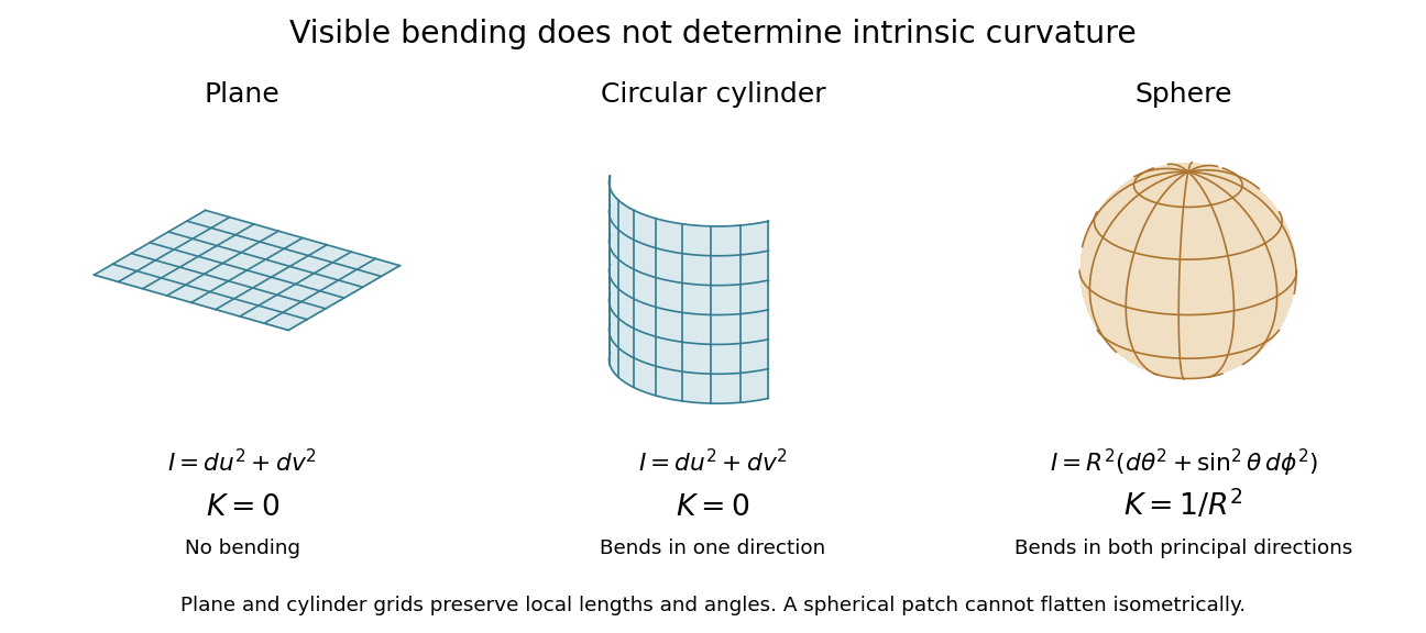
Visible bending and Gaussian curvature are different measurements
. Details. Let be a closed Riemannian manifold and a flat Hermitian vector bundle with unitary holonomy. On -valued differential forms of degree , let be the nonnegative Hodge Laplacian. For its positive eigenvalues, defineusing analytic continuation to ; the prime omits zero eigenvalues. The Ray-Singer analytic torsion isThis packages the form spectra into a regularized determinant, supplying an analytic counterpart of Reidemeister torsion.[ref]
For acyclic unitary coefficients on a closed manifold, this scalar is independent of the Riemannian metric. With nonzero cohomology, the scalar alone can depend on the metric; the full construction also tracks the norm of cohomology bases. For a circle of length with trivial coefficients, the positive eigenvalues are for in degrees zero and one. Their zeta regularization gives , illustrating that dependence.[ref]
R-torsion and the Laplacian on Riemannian manifolds by Daniel Ray and Isadore Singer. Section 2 for acyclic invariance; Section 3 for the nonacyclic construction
Turaev torsion refines the combinatorial side's sign and cellular-lift choices; comparing analytic and combinatorial constructions requires matching those conventions.
A differential 1-form is a smooth section of the cotangent bundle; it assigns a covector to every point of a smooth manifold. In planar coordinates, evaluates a tangent vector as .
Along a parametric curve , its line integral isReversing the direction reverses the integral. A force expressed as a one-form therefore accumulates work along a directed path. In Euclidean coordinates its components can be displayed as arrows, but identifying a one-form with a vector field uses an inner product; the covector field itself does not require a Riemannian metric.
For a smooth form of type , the complex orientation gives . Consequently its integral on a compact complex manifold is positive unless vanishes identically. Applying Stokes theorem to proves that a holomorphic differential form of degree on a compact complex -manifold is closed, without requiring a Kähler metric.
The comass is the operator norm of a differential form restricted to simple unit tangent multivectors. Reversing orientation gives the equivalent two-sided bound. It differs from the Euclidean norm of all the form's components. The calibration bound uses comass because tangent planes are represented by simple multivectors.
A compactly supported top-degree differential form on an oriented smooth manifold is integrated using orientation-preserving coordinates and a partition of unity. The coordinate change of variables formula makes the result independent of the choices. More generally, a form is integrated over a lower-dimensional oriented submanifold by its pullback. The Generalized Stokes theorem states with the induced boundary orientation. Integrating a closed differential form over a closed cycle depends only on its homology class, since its integral over a boundary vanishes.
A jump condition relates the one-sided limits of a solution or its derivatives across a discontinuity or singular forcing. Integrating a differential equation across a shrinking interval containing a Dirac delta source determines the permitted jump. A jump condition for an impulse and Rankine-Hugoniot condition are specific instances with different governing equations.
For the first-order ordinary differential equation defined on an open subset of the plane, an isocline of slope is the level setHere is a constant. At every point of this isocline, the direction field prescribes a tangent vector proportional to for a solution of a differential equation. It does not generally prescribe the tangent line of the isocline itself. The level set can have several components or fail to be a smooth curve, and points outside are excluded.
For example, take on the whole plane. Its isoclines are the parallel straight linesEach line has slope , while the direction field along it has slope . Thus the isocline carries horizontal segments even though the line itself rises. A function graph of a solution of a differential equation follows the segments, rather than following this line. Only the isocline with , namely , is also a solution of a differential equation.[ref]
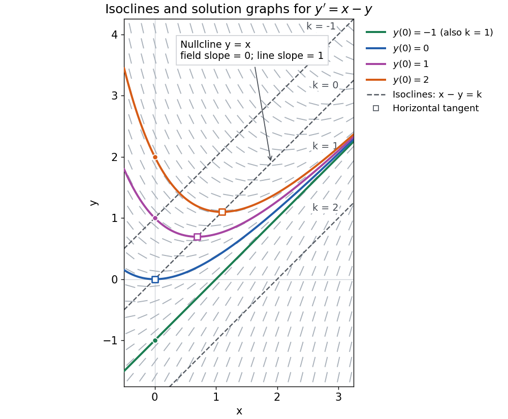
The first-order linear differential equation has the exact familyThe initial condition selects and hence a unique solution of a differential equation for every real . The picture shows . For the solution of a differential equation stays on the isocline; for other it moves through different isoclines. These formulas check the pictured trajectories by direct differentiation, independently of how the direction field was sampled.
The zero-slope isocline is called a nullcline. Below the nullcline in this example, ; above it, . For , the solution of a differential equation meets it at , where and , a strict local minimum. The nullcline is therefore a useful guide to turning points, although it is not itself a solution of a differential equation. In the equivalent planar autonomous differential equation , , it is the nullcline for the second component; there is no equilibrium point, because the first component never vanishes.
This makes isoclines useful even when no explicit solution of a differential equation is available: organize a direction field by common slopes, read where function graphs rise or fall, and identify possible turning points on nullclines.
A direction field for places a short segment with slope at each sampled point where is defined. A function graph of a solution of a differential equation follows these segments: its tangent line has exactly the prescribed slope. Segment length is a drawing choice, rather than a speed; arrows, if used, point toward increasing . An isocline collects points with one common slope.
For Newton's law of cooling, with time in minutes and temperature in degrees Celsius, the slopes at are respectively degrees Celsius per minute. Each horizontal row is an isocline, because this autonomous differential equation has no explicit time dependence. Above the solutions of a differential equation descend, below they rise, and is an equilibrium point.
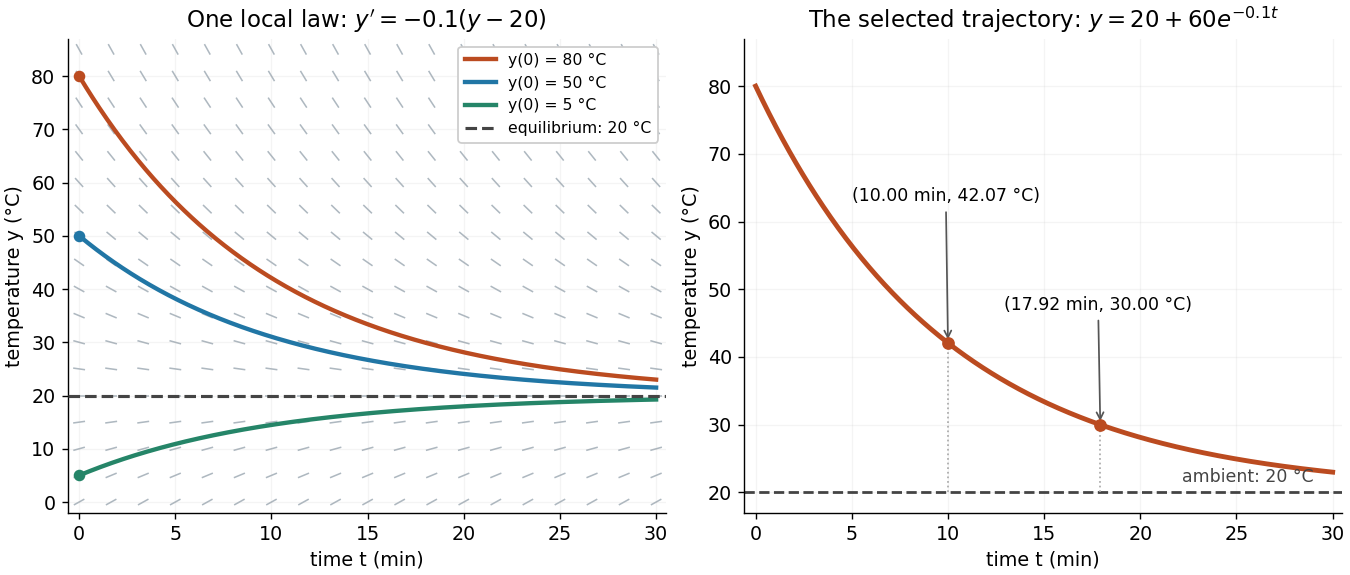
The highlighted initial condition selects one curve from the family. The picture reveals approach to the equilibrium point before any algebra is done. Under the hypotheses of the Picard-Lindelöf theorem, distinct function graphs of solutions cannot cross or even meet in the time-state plane. A direction field alone does not guarantee uniqueness: several curves can share a tangent line at the same point when those hypotheses fail. See the delayed-start example under initial value problem.
This geometric interpretation is developed in Direction Fields, Isoclines, Integral Curves.
Smoothness describes the degree of differentiability of a function. The class has continuous derivatives through order ; a smooth function is of class .
If a real function has a finite derivative at , its difference quotient tends to and is bounded for sufficiently small nonzero increments. Multiplying it by the increment shows , proving continuity at . The converse fails: the absolute value function is continuous but not differentiable at zero.
If , and both endpoints tend to , differentiability gives with . The error in the secant is bounded by for large . Thus these secants converge even when either endpoint equals .
A function with and the displayed bound has zero Fréchet derivative at zero, since . In particular, a bounded oscillatory factor multiplied by a quadratic expression is differentiable at the origin even if the oscillations have no limit themselves. For , extended by zero on the two diagonal lines, this damping works at the origin. At a nonzero point of either line, the quadratic factor instead vanishes to first order along a transverse direction; the difference quotient oscillates without a limit. Thus the differentiability set is the complement of those two lines together with the origin.
Differentiability does not imply continuity of the derivative by  Codex 0 Created 2026-10-14 Updated 2026-10-18
Extend the displayed function by . Its difference quotient at zero is , which tends to zero. Away from zero its derivative is . At this derivative equals , whereas at it equals . Thus differentiability implies continuity of the function but does not imply continuity of its derivative.
For a positive odd integer , Fermat's factorization method searches for integers satisfying . Start at and test successive values until is a perfect square . The difference of two squares then gives . For an even input, remove factors of two first.
The search always reaches at least the trivial factor pair , at . It is useful when a nontrivial factor pair is close: that pair is reached at , withA small difference between factor sizes therefore requires few trials. This is a different advantage from looking for a small prime factor by trial division.
Dielectronic capture is the resonant capture stage inverse to a specified autoionization channel. For an entrance ion of weight and resonance of weight and energy , its Maxwellian coefficient is . This follows by equating capture and autoionization fluxes at thermodynamic equilibrium. Capture alone need not produce a permanently recombined ion.
Radiative stabilization occurs when a photon emission from an autoionizing state leads to a bound state, preventing electron re-ejection. For one radiative channel and one autoionization channel, its probability is . With several channels, use summed losses and the total rate of successful stabilizing decays; a cascade through another autoionizing state requires its eventual survival probability.
Pinned article: Introduction to the OurBigBook Project
Welcome to the OurBigBook Project! Our goal is to create the perfect publishing platform for STEM subjects, and get university-level students to write the best free STEM tutorials ever.
Everyone is welcome to create an account and play with the site: ourbigbook.com/go/register. We belive that students themselves can write amazing tutorials, but teachers are welcome too. You can write about anything you want, it doesn't have to be STEM or even educational. Silly test content is very welcome and you won't be penalized in any way. Just keep it legal!
Intro to OurBigBook
. Source. We have two killer features:
- topics: topics group articles by different users with the same title, e.g. here is the topic for the "Fundamental Theorem of Calculus" ourbigbook.com/go/topic/fundamental-theorem-of-calculusArticles of different users are sorted by upvote within each article page. This feature is a bit like:
- a Wikipedia where each user can have their own version of each article
- a Q&A website like Stack Overflow, where multiple people can give their views on a given topic, and the best ones are sorted by upvote. Except you don't need to wait for someone to ask first, and any topic goes, no matter how narrow or broad
This feature makes it possible for readers to find better explanations of any topic created by other writers. And it allows writers to create an explanation in a place that readers might actually find it.
Figure 1. Screenshot of the "Derivative" topic page. View it live at: ourbigbook.com/go/topic/derivativeVideo 2. OurBigBook Web topics demo. Source. - local editing: you can store all your personal knowledge base content locally in a plaintext markup format that can be edited locally and published either:This way you can be sure that even if OurBigBook.com were to go down one day (which we have no plans to do as it is quite cheap to host!), your content will still be perfectly readable as a static site.
- to OurBigBook.com to get awesome multi-user features like topics and likes
- as HTML files to a static website, which you can host yourself for free on many external providers like GitHub Pages, and remain in full control

Figure 2. You can publish local OurBigBook lightweight markup files to either OurBigBook.com or as a static website.
Figure 3. Visual Studio Code extension installation.
Figure 5. . You can also edit articles on the Web editor without installing anything locally. Video 3. Edit locally and publish demo. Source. This shows editing OurBigBook Markup and publishing it using the Visual Studio Code extension. 
- Infinitely deep tables of contents:




All our software is open source and hosted at: github.com/ourbigbook/ourbigbook
Further documentation can be found at: docs.ourbigbook.com
Feel free to reach our to us for any help or suggestions: docs.ourbigbook.com/#contact