Topics (384k) Articles (398k) Users (410) Discussions (242) Comments (383) Files (13k) New article

Relative to a propagation plane, transverse magnetic polarization has its magnetic field perpendicular to that plane. At a perfectly conducting corrugation its scalar magnetic component obeys a Neumann condition. It reduces to a scalar two-dimensional problem, but not to the Dirichlet problem for the transverse electric component.
Take a straight hollow rectangular electromagnetic waveguide with vacuum interior , and axis , where . Its four walls are ideal perfect conductors. The time-dependent Maxwell equations require zero tangential electric field and zero normal oscillating magnetic field at these walls. Real metal has finite electrical conductivity, so real guides lose electromagnetic energy by Joule heating; the perfect-wall model isolates confinement and wave dispersion from that loss.
The simplest propagating transverse electric mode of a rectangular waveguide is . “Transverse electric” means , not that the magnetic field is also wholly transverse. With real peak scale , its complex amplitudes, including the common axial factor, can be writtenThe physical fields are the real parts after multiplication by . In particular, is zero at , maximal at , and independent of . At it is normal to the metal, so it need not vanish there. The electric field crosses the narrow gap, while its strength varies across the broad dimension.
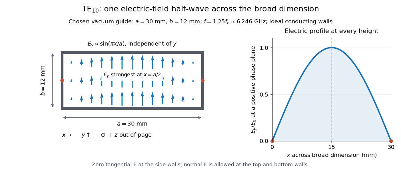
Original vacuum-filled rectangular guide: the TE10 electric-field profile across a 30 mm by 12 mm cross-section
. The arrows show the electric field at an axial plane and time where its common wave phase factor is positive; their length follows . They are field directions, not particle trajectories. The profile is uniform along and vanishes at the side walls. The guide axis points out of the cross-section. All dimensions and the operating frequency are chosen model values. Details.For an original example choose , and , where . With , this givesHere is vacuum wavelength and is guided wavelength. The next cutoff is at ; starts at . Thus only can propagate at the chosen frequency, although a source or discontinuity can additionally excite local evanescent waves. These are calculated values, not specifications or measurements of a commercial guide.
An electromagnetic waveguide confines an electromagnetic wave across its axis while allowing it to travel along the axis. Conducting walls or changes of refractive index select transverse normal modes: reproducible cross-sectional field patterns with their own longitudinal wavenumbers. A hollow metal pipe and an optical fiber are different realizations of this principle. Their usefulness is to deliver electromagnetic energy along a chosen route instead of letting it spread freely.
For a uniform vacuum-filled conducting guide, write a normal mode's axial and time dependence as . Here is angular frequency, is the longitudinal wavenumber, and is the transverse eigenvalue selected by the wall boundary conditions. The electromagnetic wave equation separates intoThe geometry consumes part of the available squared wavenumber: when , this branch is an evanescent wave rather than a propagating normal mode. The waveguide cutoff frequency is therefore a property of a specified branch and geometry. A transverse electromagnetic mode in a suitable two-conductor geometry can have and no positive geometric cutoff. An optical fiber needs its own dielectric boundary conditions, rather than the metal-wall formulas below.
The rectangular electromagnetic waveguide makes these ideas explicit with a single sine profile. The scalar-potential conducting waveguide modes give a broader construction. At an open aperture, a confined field can radiate into the electromagnetic aperture angular spectrum; it need not remain one guided normal mode.
For a sphere of radius , the scattering efficiency is its effective scattering area divided by the projected geometric cross-section . It is a dimensionless quantity. For Rayleigh scattering by a small sphere with relative refractive index and incident wavenumber ,At fixed wavelength and fixed refractive index, the Rayleigh scattering cross-section scales as , whereas the scattering efficiency scales as . Doubling radius multiplies the former by and the latter by . An efficiency here is an effective scattering area relative to a reference area, rather than a fraction of all light in an arbitrary beam.
For a worked toy example, take , , and . Then and . Substitution gives Rayleigh scattering cross-section and scattering efficiency . At incident light intensity , the scattered power is approximately . These are leading small-particle estimates, not a measured air-molecule cross-section.
X-rays are high-frequency electromagnetic radiation, conventionally with wavelengths of roughly to . The precise wavelength convention varies with context. Hot accreting gas and energetic electronic processes can emit X-rays, whose short wavelengths make them useful probes of compact objects and electron shells.
For a photon, , where is the Planck constant and is the speed of light. As a calculated example, gives , using . The same wavelength can describe different production mechanisms: bremsstrahlung produces a continuous frequency spectrum, whereas Characteristic X-rays arise from discrete electronic changes in chemical atoms. Measuring transmitted X-rays gives radiography; measuring their frequency spectrum gives spectroscopy.
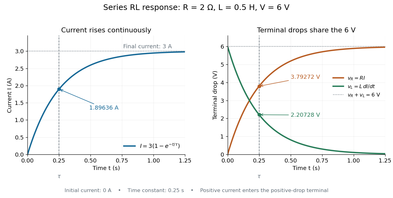
An RL circuit combines electrical resistance and self-inductance . In the series model, the same electric current flows through both components. An ideal battery maintains terminal electric potential difference ; the drops in the direction of positive electric current obey Ohm's law and the inductor relation:This is Kirchhoff's voltage law with the inductor's terminal drop, rather than its oppositely signed induced electromotive force. For constant , , and , the first-order linear differential equation has solutionThe time constant measures exponential decay of the difference from the final electric current. [ref].
For a stipulated example, take electrical resistance , self-inductance , terminal electric potential difference , and initial electric current . ThenWith measured numerically in seconds, this is in amperes. At one time constant,and the terminal electric potential difference drops areTheir sum is exactly . At , the inductor takes the entire terminal electric potential difference while the electric current is still zero. At steady electric current, the inductor's terminal drop is zero and the entire drop is across the electrical resistance.
The final magnetic energy stored by the inductor is . At one time constant, the electric current has reached about of its final value, but its magnetic energy has reached only about :This difference follows from the square of electric current in the inductor's magnetic energy.
For release, take at the start of a separate experiment with initial electric current . Remove the battery from the model while maintaining a closed path through the same electrical resistance and inductor. ThenNow : the induced electromotive force supports the continuing positive electric current as its magnitude decreases. This closed-loop model describes exponential decay, not opening the sole path and imposing an instantaneous jump to zero electric current. The inductor's magnetic energy and the power of Joule heating areTheir time constant is . The total energy dissipated by Joule heating is exactly the initial magnetic energy:The second diagram in inductor shows this energy transfer. A finite closed path lets us predict both how long the electric current persists and how much energy becomes heat. [ref]
https://openstax.org/books/university-physics-volume-2/pages/14-4-rl-circuits. OpenStax University Physics 2, §14.4: decay in a closed RL loop
.An electric battery converts the available chemical Gibbs free energy of one or more galvanic cells into electrical work delivered to an electrical load. The reacting materials are a finite reservoir: a battery can sustain a terminal electric potential difference while discharging, but cannot supply energy indefinitely. Unlike a capacitor, whose capacitor energy resides in an electric field, a battery chiefly stores its available energy in the chemical state of its materials. The detailed half-reactions and apparatus of a Daniell cell explain this conversion at the electrode level.
During discharge, electrons move through metallic wires from the negative anode, through the electrical load, to the positive cathode; external conventional current points the other way. Inside the battery, ions carry electric current through the electrolyte, and redox chemical reactions connect ionic transport to electronic transport at the electrodes. The same electron does not make a lap through both wire and electrolyte. Electric charge conservation closes the circuit; changing chemical composition supplies the energy. See galvanic cell for the two transport paths and electrolyte for how oppositely moving ions contribute to one net electric current.
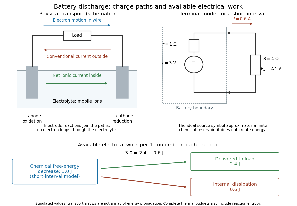
The source's electromotive force measures its driving work per unit electric charge, in volts; the loaded terminal electric potential difference measures the electrical work per unit electric charge delivered outside the battery. They agree in an ideal lossless source, or approximately near open circuit, but generally differ during discharge.[ref]
University Physics Volume 2 by Samuel J. Ling and others. §10.1, Introduction to Electromotive Force, work per charge and terminal voltage
In the ideal fixed-voltage model used in fixed-voltage capacitor energy balance, a battery maintains a prescribed terminal electric potential difference while electric charge flows to or from the capacitor. This is a constraint for that calculation, not an inexhaustible reservoir. The fixed-voltage capacitor energy balance also accounts for electrical energy returned to the source; an actual cell can accept sustained charging only if its chemistry and operating conditions permit it.
Electrical impedance is the ratio of terminal electric potential difference and electric current phasors at one specified positive angular frequency . For an electrical circuit modeled as a linear time-invariant system, use the sinusoidal steady state after any decaying transient has settled. With the passive sign convention, positive electric current enters the terminal assigned positive electric potential difference. Define peak complex amplitudes byThe physical and are real; the complex numbers encode their amplitudes and wave phases. The unit of electrical impedance is the ohm, . Both phasors may instead use root mean square magnitudes, with the same ratio . A nonlinear diode can generate additional frequencies; a single then does not describe the whole response.
Write the electrical impedance in Cartesian and polar forms asHere is the resistive real part, the signed electrical reactance, and the voltage-minus-current phase difference, defined modulo a full turn. The Pythagorean theorem gives the modulus from a right triangle in the complex plane. The complex argument gives the rotation from the current phasor to the voltage phasor. Thus , while negative means electric current leads terminal electric potential difference. For , lies between and ; outside that case, use the quadrant of the complex number rather than a bare inverse tangent. The geometric magnitude and phase difference are the two pieces of the AC relation.[ref]
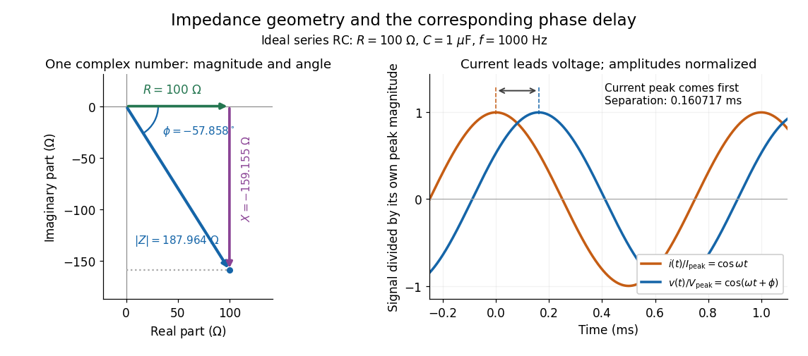
Multiplication by acts on phasors, not on instantaneous physical signals. For example, when ,The second term is in phase quadrature with electric current; it cannot be represented by pointwise multiplication when . This is the useful compression: one complex multiplication replaces separate amplitude and phase difference calculations, while the real part restores the physical signal.
An ideal resistor, inductor and capacitor have , and . Their electrical impedances add in a series RLC circuit, giving . The current amplitude is , so cancellation of the imaginary parts explains the resonant series RLC response. The component-law derivation and opposite complex exponential convention are in reactance phase convention.
The passive sign convention defines terminal electric potential difference and positive electric current entering at . Then is absorbed electrical power: positive means the component receives energy, negative means it supplies energy. Reversing both reference directions leaves the product unchanged. For a positive electrical resistance obeying Ohm's law, both and reverse together and Joule heating remains .
Electric flux measures how much electric field crosses a chosen oriented surface, with a sign distinguishing the two crossing directions. A strong electric field running along a surface contributes nothing to its electric flux: only the normal component counts. This lets Gauss's law turn a potentially complicated electric field into one number recording the net enclosed electric charge.
For a surface with chosen unit normal , the electric flux is the surface integralHere is positive surface area, while is the vector area element. The dot product makes electric flux a signed scalar, rather than a vector like the electric field. Its SI unit is : electric field measured using the newton per coulomb, multiplied by surface area in square metres. Reversing the orientation of a surface replaces by and reverses the electric flux. Calling it electric flux does not imply that electric charge is moving through the surface. [ref]
https://www.feynmanlectures.caltech.edu/II_03.html#Ch3-S2. Feynman lectures II.3, §3–2: flux of a vector field
.For an open patch in a plane, with surface area and a constant electric field, the unit normal is constant and the surface integral simplifies toThe angle is between the electric field and the chosen unit normal, not between the electric field and the plane. The cosine describes the signed projected surface area seen by the electric field. Thus electric flux is positive for , zero at , and negative for . [ref]
https://openstax.org/books/university-physics-volume-2/pages/6-1-electric-flux. Ling, Sanny and Moebs, University Physics II, §6.1: electric flux
.For example, take and , so . Three choices of angle giveKeeping the patch fixed and reversing its unit normal gives and changes to . The electric field and physical patch have not changed. If the electric field is instead tangent to the patch, its dot product with the unit normal vanishes: electric flux is zero even though .
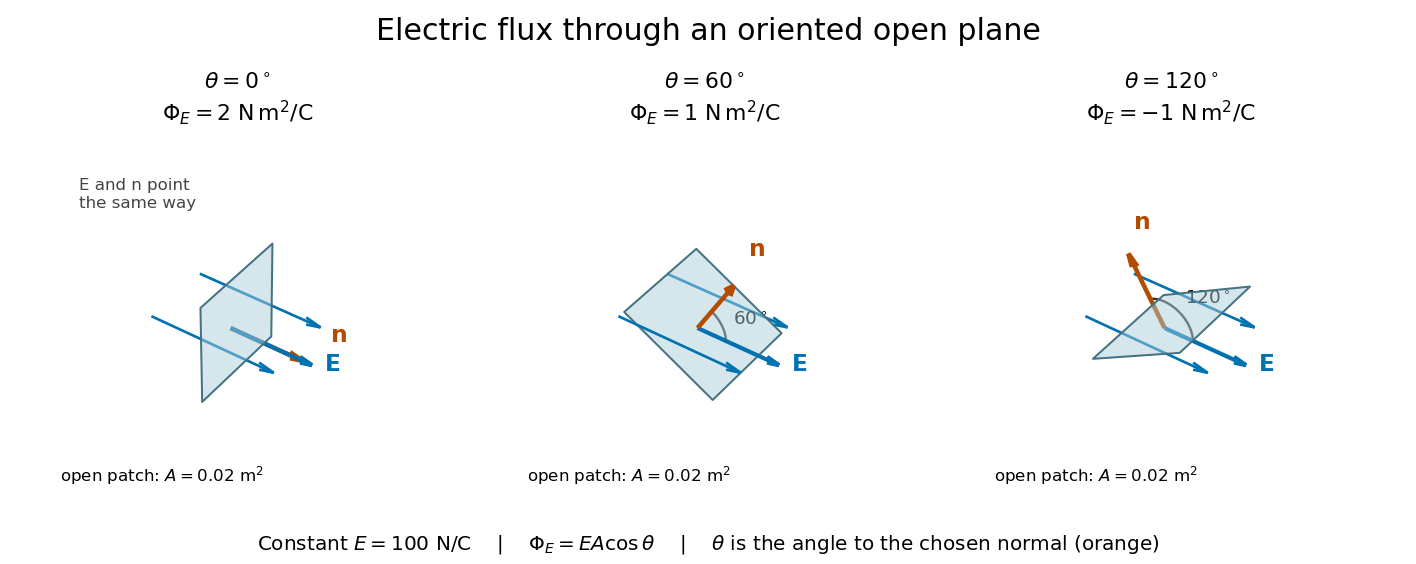
Three open patches in a plane in a constant electric field: the angle to the chosen unit normal gives electric fluxes of 2, 1 and minus 1 newton square metres per coulomb
. Details. For a closed surface enclosing a volume , choose the outward unit normal. Gauss's law givesHere is the vacuum permittivity, and is the signed total electric charge inside. The electric field in the surface integral includes all sources, including external electric charges. Assume no ideal point charge lies on the integration surface. Zero enclosed electric charge implies zero total electric flux; it does not imply zero electric field everywhere on the closed surface or inside it. Positive and negative contributions to the surface integral can cancel. [ref]
https://openstax.org/books/university-physics-volume-2/pages/6-2-explaining-gausss-law. Ling, Sanny and Moebs, University Physics II, §6.2: outward flux and enclosed charge
.To see the cancellation with sources inside, place point charges at and at , where , , and both lie inside the sphere of radius centered at the origin. This separated pair has the electric dipole geometry. Its enclosed electric charge is , so its total outward electric flux is zero. At the point on the sphere, Coulomb's law and the superposition principle give the individual electric fieldsThe components cancel and the positive components add:For the stipulated approximation and , this is about along positive . At , the outward unit normal is , so this nonzero electric field is tangent to the sphere. At other points of the sphere, its normal component can be positive or negative. The source-field formula applies away from the two point charges, where the electric field has zero divergence; it is singular at the sources. [ref]
https://www.feynmanlectures.caltech.edu/II_04.html#Ch4-S2. Feynman lectures II.4, §§4–1 and 4–2: electrostatic sources and superposition
.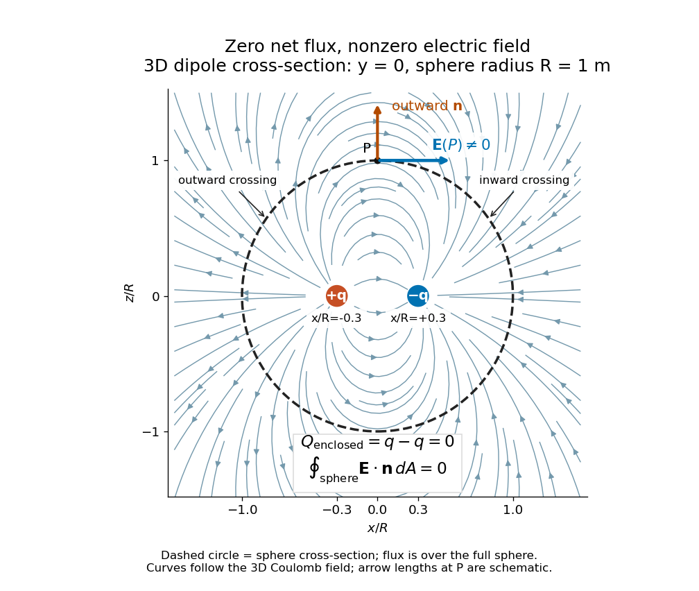
Cross-section of the three-dimensional electric field of two opposite point charges inside a unit-radius sphere: zero total electric flux coexists with a nonzero tangential electric field at the top
. Details. The diagram shows streamlines of the three-dimensional electric field in the section . The circle is a cross-section of the sphere, not the integration surface: Gauss's law uses the entire three-dimensional surface integral. A two-dimensional line integral of outward field around that circle would be a different quantity, with units rather than the electric flux units .
The electric force on an electric charge is , using the electric field of the other sources and excluding the charge's own self-field. Positive electric charge gives force along the electric field; negative electric charge reverses it. A field therefore gives on . This is the electric part of the Lorentz force; the magnetic contribution is . [ref].
Charge conservation says that the total signed electric charge of an isolated collection stays constant. More generally, a collection closed to electric charge exchange has constant total electric charge, even if energy crosses its boundary. This is the charge bookkeeping relevant to a closed system or an isolated system; isolation from energy exchange is not required. Positive and negative electric charge count with opposite signs. Creating or removing an electron and a Positron together is compatible with charge conservation, because their combined electric charge is zero. [ref]
https://www.feynmanlectures.caltech.edu/I_04.html#Ch4-S4. Feynman, Leighton and Sands, The Feynman Lectures on Physics, I.4.4: net charge conservation
.Imagine a fixed box initially containing electric charge . Stipulate incoming conventional current and outgoing conventional current throughout , with no other boundary transport. Since one ampere is one coulomb per second, the stored electric charge grows at :If instead the outgoing electric current also equals , the stored electric charge remains while electric charge passes through. These are stipulated transport examples; constant terminal electric currents alone do not guarantee a time-independent interior charge density.
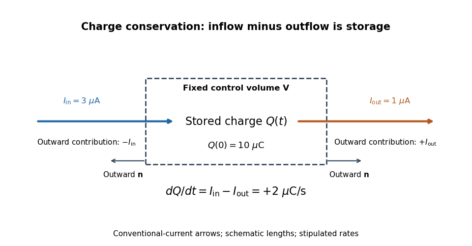
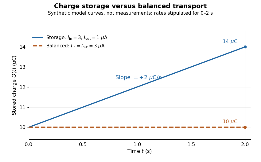
Stored electric charge with unequal and balanced terminal electric currents
. Synthetic curves from the stipulated rates over , with the same initial electric charge; these are not measurements. Balanced transport keeps total electric charge fixed, and is compatible with steady transport. Source. Details.Locally, charge conservation is the charge continuity equation, an instance of the general continuity equation:Here is signed volume charge density and is current density. A positive divergence of current density means net outward transport from a small neighborhood, so its charge density decreases. For a fixed control volume with closed surface and outward unit normal , the equivalent integrated balance isThe surface integral is signed: incoming positive electric charge contributes negatively to outward electric current, and outgoing positive electric charge contributes positively. Integrate the charge continuity equation over fixed and apply the divergence theorem to obtain this balance. Zero net boundary transport gives constant ; the global and local statements describe the same conservation law at different scales. [ref]
https://www.feynmanlectures.caltech.edu/II_13.html#Ch13-S2. Feynman, Leighton and Sands, II.13.2: local and integrated charge conservation
.In a steady transport state, charge density and current density are time-independent, so the charge continuity equation reduces to . At an electrical circuit junction, choose each terminal electric current positive outward and assume the terminals account for all boundary transport. ThenKirchhoff's current law, , follows when accumulation of electric charge at the junction is negligible. During storage, retain the same balance with its nonzero derivative; charge conservation continues to hold. This makes charge conservation useful for checking electrical circuit models and for tracking the charging of a capacitor. [ref]
https://openstax.org/books/university-physics-volume-2/pages/10-3-kirchhoffs-rules. Ling, Sanny and Moebs, University Physics II, §10.3: Kirchhoff's junction rule
.The beautiful consistency with Maxwell equations is that the electric field and magnetic field already enforce this transport balance. For sufficiently smooth fields in vacuum SI, take the divergence of the Ampère-Maxwell equation, use that the divergence of a curl is zero, and substitute Gauss's law, . Constant vacuum permittivity givesThe displacement current term supplies the part needed when electric charge accumulates. Historically, Maxwell added that term to extend the steady-current equation; see the existing charge conservation from Maxwell equations for this connection. [ref]
https://www.feynmanlectures.caltech.edu/II_18.html#Ch18-S1. Feynman, Leighton and Sands, II.18.1: Maxwell's added term and charge conservation
.Electrostatic induction is redistribution of electric charge in response to an external charged object. An isolated electrical conductor can acquire positive and negative surface regions while its total electric charge stays fixed; see the contact control in electric charge.
An electrometer measures small electric potential differences or electric charges while drawing very little electric current. The conducting-pail experiment in electric charge uses a voltage response to infer electric charge with a fixed effective capacitance.
The elementary charge is the positive magnitude of the electron's electric charge, not the signed electric charge of the electron itself:Since the 2019 revision of the SI, this numerical value defines the ampere together with the definition of the second; . Thus today's numerical exactness is a choice of units, whereas measured electric charges still have experimental uncertainty. An oil drop experiment can test charge quantization and the apparatus calibration; it does not supply a new uncertain defining value of in today's SI. [ref]
https://www.bipm.org/documents/20126/41483022/SI-Brochure-9-EN.pdf. BIPM, The International System of Units, ninth edition, sections 2.2 and 2.3.1, the ampere
.For ordinary isolated chemical atoms, ions and charged objects whose net electric charge is counted through protons and electrons, charge quantization gives with signed integer . A neutral chemical atom that loses two electrons becomes an ion of electric charge . A toy object with excess electrons has . Conversely, the scale explains why laboratory electric charge often looks continuous: billions of microscopic increments fit into a small macroscopic amount. Averaged charge density is a continuum description, not a claim that each particle has an arbitrarily divisible electric charge.
The ordinary-matter qualifier matters. In the Standard Model, quarks have electric charges or , and antiquarks have the opposite signs. Confinement means these are constituents of hadrons, not isolated fractionally charged particles collected by an oil drop experiment. The usual valence quark sums give for a proton and for a neutron. Thus elementary charge should not be defined as the smallest nonzero electric charge of every constituent in particle theory. [ref]
https://pdg.lbl.gov/2022/reviews/rpp2022-rev-quark-model.pdf. Amsler, DeGrand and Krusche, Particle Data Group, Quark Model, sections 15.1–15.2 and table 15.1
.The beautiful experimental idea behind the oil drop experiment is to determine a microscopic electric charge by watching a visible carrier move. In his 1913 paper, Millikan timed the descent and electrically driven ascent of individual oil drops, repeatedly changing a drop's electric charge through capture of air ions. His apparatus used parallel plates separated by , a roughly source, and an optical scale to measure travel distances. He reported multiple relationships among a given drop's inferred electric charges. He also found that uncorrected Stokes's law gave a size-dependent inferred elementary unit, and introduced a pressure-dependent slip correction. These were measured relationships with calibration and model uncertainties, not exact readings of today's defined . [ref]
https://grundpraktikum.physik.uni-saarland.de/gpalt/Anleitungen/Ergaenzungen/Versuche/Millikan/Millikan%20-%20On%20the%20Elementary%20Electrical%20Charge%20and%20the%20Avogadro%20Constant.pdf. R. A. Millikan, On the Elementary Electrical Charge and the Avogadro Constant, Physical Review 2 (1913), 109–143, especially pp. 109–112 and 115–116
.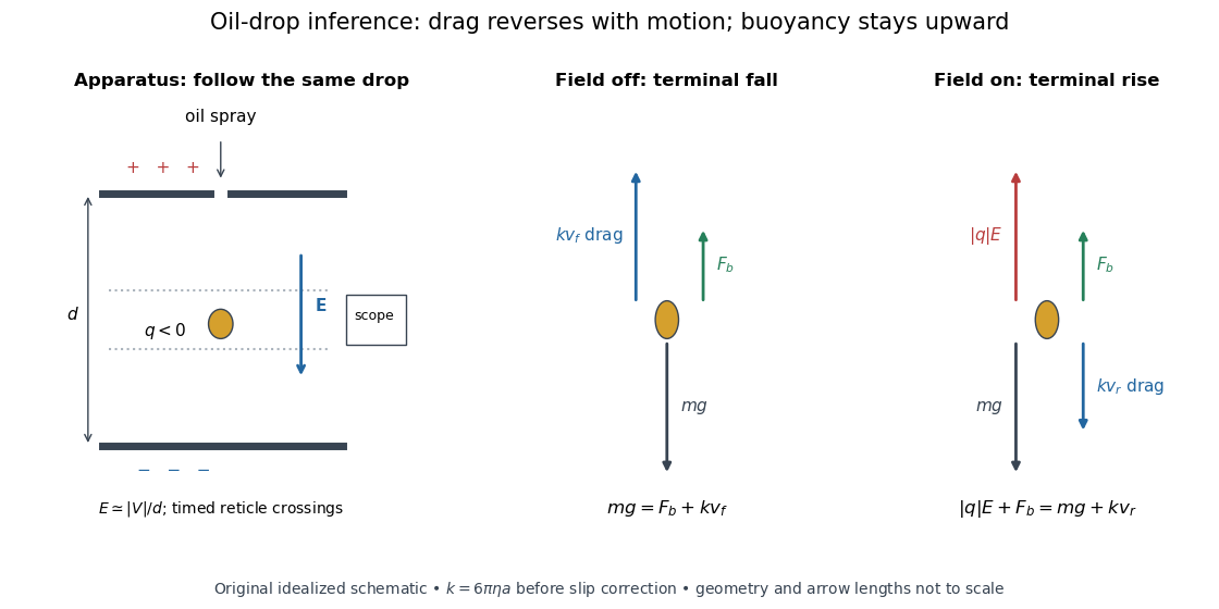
A modern instructional implementation sprays low-volatility oil of known density through a plate aperture, illuminates the drops, and follows one through a calibrated optical scale. Measure the plate spacing , electric potential difference , air temperature and pressure. Time a fixed distance with the electric field off to get a terminal falling speed . Then choose the field polarity to drive the same drop upward and measure . Repeat timings at a fixed electric charge, and compare before and after an ion-capture event. The same drop is especially useful because its radius and mass need not be inferred anew for each charge state. [ref]
https://cdn.pasco.com/product_document/Millikan-Oil-Drop-Manual-AP-8210B.pdf. PASCO, Millikan Oil Drop Apparatus AP-8210B manual, introduction, theory and experimental procedure
.Here is the leading continuum model, retaining buoyancy. Assume a drop shaped as a sphere of radius , oil and air densities and , air dynamic viscosity , and gravitational acceleration . Define the downward effective weight and positive linear drag coefficient byAt terminal velocity, the net force vanishes. Falling with no electric field, the upward drag force balances weight minus buoyancy. Rising with the electric force upward, the drag force reverses and joins the downward effective weight:Consequently the uncorrected estimates areThe observed direction of response, with known field polarity, supplies the sign of . A suspended drop gives the alternative balance , but it still requires a determination of : balancing a drop alone does not determine its electric charge.
For an explicitly invented continuum example, stipulate , , , , , and a downward . The balances predict , and . Substituting those speeds recovers within rounding. This checks the algebra; it is not a precision prediction for real micrometre drops, which need a slip correction.
The inference has two distinct parts. Compare inferred electric charges or charge changes with a common unit, seeking within uncertainty, rather than demanding exact ratios of rounded measurements. Then establish the absolute scale through electric field, density, dynamic viscosity and distance/time calibration. If the observed steps are all even multiples, their common spacing alone cannot exclude an unobserved smaller unit. Air motion, evaporation and mistimed crossings can alter inferred electric charge without an ion-capture event. Small Reynolds number supports Stokes's law, but does not by itself justify its no-slip continuum coefficient: a significant ratio of air mean free path to drop radius requires a slip correction. Millikan's comparison of different drop sizes and pressures addressed that systematic limitation; the modern PASCO manual also includes the correction. Agreement supports charge quantization for the observed carriers within experimental resolution, rather than proving a universal statement about every possible particle.
Multiplying by the Avogadro constant gives the Faraday constant, , the electric charge per mole of singly charged carriers. This connects counting individual electric charges with bulk electrochemistry. [ref]
https://physics.nist.gov/cuu/pdf/wall_2022.pdf. NIST, CODATA 2022 defining constants and Faraday constant
.Finite elasticity describes reversible deformations without assuming that stretches or rotations are small. A material point initially at moves to , with deformation gradient . A useful measure of local stretching is the Green-Lagrange strain tensor,For a pure rotation, is an orthogonal matrix and : rotating a specimen does not stretch it. This property is essential when, for example, a thin elastic rod bends through a large angle.
Both geometry and the constitutive equation matter. Current area and volume can differ substantially from their values in the reference configuration, and different stress tensors refer to different areas. A hyperelastic material supplies the response through a strain energy density. Rubber stretching and large bending motivate this framework even when the specimen returns to its original shape on unloading; large reversible deformation does not imply plastic deformation.
The shear modulus is the ratio of shear stress to small engineering shear strain in an isotropic linear elastic material:For a slab of thickness whose upper face moves sideways by while the lower face is fixed, . A tangential force distributed over face area gives . Thus in the uniform-shear idealization. Its units are pressure, and the engineering convention gives in terms of the infinitesimal strain tensor.
An experiment on the torsion of a solid circular shaft measures the same parameter through torque and end rotation: for shaft length and polar second moment of area , . This separates material resistance to shear strain from the specimen's geometric resistance to twisting. In isotropic linear elasticity, , where is Young's modulus and is Poisson's ratio.
For two Fourier elastic wave fields with the same real elastic stiffness tensor, its major symmetry cancels the cross-strain terms in the divergence displayed above. The force-balance equations supply the remaining volume terms, and the divergence theorem gives their boundary integral of reciprocal tractions. Taking one field to be a complex conjugate gives energy-work identities and weighted modal orthogonality. The bilinear identity uses no complex conjugation until that field is chosen explicitly.
Magnetostriction is a change of a material's shape or dimensions associated with its magnetization. A magnetic field can therefore produce strain without a contact force. The resulting magnetoelastic coupling lets a ferromagnet convert changes of magnetic state into mechanical motion; a constraint can instead turn the preferred deformation into stress. James Prescott Joule published his study of iron and steel bars in 1847.[ref]
The surprising point is that reversing the magnetization need not reverse the deformation. A material can prefer a longer axis along either or : an axis has no arrow. Isotropic linear magnetostriction vanishes excludes one particular linear constitutive term, while saturated isotropic magnetostrictive strain supplies a nonzero response with a quadratic dependence on the magnetic direction. The pulsed-field optical magnetostriction experiment shows how an actual length change can be resolved, and quadratic magnetostriction and frequency doubling separates an illustrative response law from a measured material curve.
In an elastic boundary value problem, a dead load is a prescribed force independent of the incremental displacement. A dead reference traction has , even when the current face changes orientation. This differs from a follower load, whose direction follows the moving body, and from the structural-engineering use of the same phrase for permanent self-weight. Under pure dead tractions, a constant incremental translation remains a zero-frequency mode unless a displacement condition fixes it.
Pinned article: Introduction to the OurBigBook Project
Welcome to the OurBigBook Project! Our goal is to create the perfect publishing platform for STEM subjects, and get university-level students to write the best free STEM tutorials ever.
Everyone is welcome to create an account and play with the site: ourbigbook.com/go/register. We belive that students themselves can write amazing tutorials, but teachers are welcome too. You can write about anything you want, it doesn't have to be STEM or even educational. Silly test content is very welcome and you won't be penalized in any way. Just keep it legal!
Intro to OurBigBook
. Source. We have two killer features:
- topics: topics group articles by different users with the same title, e.g. here is the topic for the "Fundamental Theorem of Calculus" ourbigbook.com/go/topic/fundamental-theorem-of-calculusArticles of different users are sorted by upvote within each article page. This feature is a bit like:
- a Wikipedia where each user can have their own version of each article
- a Q&A website like Stack Overflow, where multiple people can give their views on a given topic, and the best ones are sorted by upvote. Except you don't need to wait for someone to ask first, and any topic goes, no matter how narrow or broad
This feature makes it possible for readers to find better explanations of any topic created by other writers. And it allows writers to create an explanation in a place that readers might actually find it.
Figure 1. Screenshot of the "Derivative" topic page. View it live at: ourbigbook.com/go/topic/derivativeVideo 2. OurBigBook Web topics demo. Source. - local editing: you can store all your personal knowledge base content locally in a plaintext markup format that can be edited locally and published either:This way you can be sure that even if OurBigBook.com were to go down one day (which we have no plans to do as it is quite cheap to host!), your content will still be perfectly readable as a static site.
- to OurBigBook.com to get awesome multi-user features like topics and likes
- as HTML files to a static website, which you can host yourself for free on many external providers like GitHub Pages, and remain in full control

Figure 2. You can publish local OurBigBook lightweight markup files to either OurBigBook.com or as a static website.
Figure 3. Visual Studio Code extension installation.
Figure 5. . You can also edit articles on the Web editor without installing anything locally. Video 3. Edit locally and publish demo. Source. This shows editing OurBigBook Markup and publishing it using the Visual Studio Code extension. 
- Infinitely deep tables of contents:




All our software is open source and hosted at: github.com/ourbigbook/ourbigbook
Further documentation can be found at: docs.ourbigbook.com
Feel free to reach our to us for any help or suggestions: docs.ourbigbook.com/#contact