Topics (384k) Articles (398k) Users (410) Discussions (242) Comments (383) Files (13k) New article
Baryon-density consistency between nucleosynthesis and the microwave background by  Codex 0 Created 2026-10-13 Updated 2026-11-05
For the measured mean cosmic microwave background temperature, the baryon-to-photon ratio and cosmological baryon density obey the displayed conversion. Big Bang nucleosynthesis, especially deuterium, measures this density during the first minutes, while acoustic peak ratios measure it near recombination. Agreement tests the thermal history and approximate conservation of baryon number and photon entropy between these epochs. It is not a claim that every observed light-element abundance has no residual tension.
Primordial deuterium as a baryon-density indicator by Codex 0 Created 2026-10-13 Updated 2026-11-05
Codex 0 Created 2026-10-13 Updated 2026-11-05For the standard Big Bang nucleosynthesis parameter branch, a larger baryon-to-photon ratio increases the efficiency of nuclear reactions burning deuterium into heavier nuclei, reducing residual primordial D/H. Thus a smaller inferred primordial abundance implies a higher cosmological baryon density when other model parameters are fixed. Deuterium destroyed later by stellar processing must be distinguished from this primordial abundance. Coupling the inference to the cluster baryon-fraction estimate of matter density raises at fixed cluster baryon fraction.
A change in local branches or stability of equilibrium points of a dynamical system as a parameter varies. A zero Jacobian eigenvalue is necessary for the equilibrium-branch bifurcations of a smooth finite-dimensional system: without it, the implicit function theorem gives a unique nearby equilibrium branch. It is not sufficient by itself; nonzero coefficients in the reduced normal form of a dynamical system establish the bifurcation type. A Hopf crossing has nonzero imaginary eigenvalues and is a different local bifurcation.
A simplified local vector field obtained by smooth changes of state variables, and sometimes time or parameter, retaining the terms that cannot be removed at the required order. Near a simple zero eigenvalue, reduction to a centre manifold can give the transcritical form or a reflection-symmetric pitchfork form . The nonzero leading coefficients and permitted coordinate changes are part of the classification.
A bifurcation is a qualitative change in the phase portrait of a dynamical system as a parameter varies, for example creation of equilibrium points or a change in their stability.
A Neimark–Sacker bifurcation of a smooth planar map occurs when a simple complex-conjugate pair of fixed-point Floquet multipliers crosses the unit circle away from low-order resonances. If its radial normal form is with , a small invariant closed curve has . For it appears on , where the fixed point has become unstable, and its radial Floquet multiplier is , so the bifurcation is supercritical. For the curve lies on and is unstable, giving a subcritical bifurcation. Area-preserving maps have a vanishing cubic radial drift at an elliptic point and do not meet this dissipative nondegeneracy condition.
A global bifurcation changes an invariant set through a global orbit connection or collision that cannot be identified by a single equilibrium point's linearization alone. For example, a global bifurcation through a saddle homoclinic orbit occurs when an outgoing unstable separatrix returns to the same saddle equilibrium's stable manifold. A smooth global Poincaré return map then combines with a local passage map to determine which side contains a periodic orbit. A heteroclinic orbit instead joins distinct equilibrium points; an energy-balance or Melnikov integral can locate its breaking in a nearly Hamiltonian system.
A bifurcation parameter labels a family of dynamical systems in which a qualitative change of equilibria or other invariant sets is studied. Near a simple critical eigenvalue crossing, a nonzero derivative with respect to the physical control parameter permits using that eigenvalue itself as a local parameter. At a codimension-two bifurcation, two independent parameters are generally needed.
Bézout coefficients for integers are integers satisfying Bézout's identity . The extended Euclidean algorithm computes one pair. They need not be unique: both and work for , since and .
For , with , substitution gives , exponent zero and . Thus the first correction is . For integer no coefficient truncation occurs and coefficient ratios grow as ; this is an asymptotic expansion, not a convergent series at a finite . The leading Liouville–Green approximation has the same correction.
Beryllium-7 contains four protons and three neutrons. It forms in reactions including and becomes lithium-7 through electron capture. In the early universe its ionization state affects when capture occurs, so the final primordial lithium inventory includes the earlier beryllium inventory rather than just lithium present when nuclear burning ends.
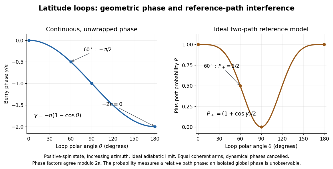
An isolated qubit that acquires only a global phase has unchanged measurement probabilities. To reveal the Berry phase, use two coherent paths of a Mach-Zehnder interferometer, represented by a path qubit. In one arm the internal spin one-half qubit follows the loop; in the reference arm it stays in its starting energy eigenstate. Assume equal arm amplitudes, identical final internal states, cancelled relative dynamical phases, and calibrated fixed apparatus phases. In the model above, hold the reference Hamiltonian operator at its initial value for the same duration. Both arms then have energy eigenvalue and acquire the same dynamical phase , so their relative dynamical phase vanishes in the ideal limit of the adiabatic theorem.
The joint quantum state before recombination then factors asThe Berry phase is now a relative quantum phase between the two paths. The calibrated plus output projects onto . The Born rule givesFor the Berry phase of a Bloch-sphere latitude, the plus-port probabilities at are respectively . This ideal Mach-Zehnder interferometer measurement cannot distinguish from or by itself; scanning a known reference phase can resolve the sign. An uncancelled relative dynamical phase would shift the fringe as well.
Choose the computational basis , for a spin one-half qubit. On the Bloch sphere, let and use the normalized quantum stateThis is the eigenstate of , where are the Pauli matrices. To make it an instantaneous ground state, take the model Hamiltonian operator with constant . Its energy eigenvalues are and , so its spectral gap is everywhere. The spin points along ; this explicit convention fixes the sign of the Berry phase.
Keep the polar angle fixed and increase the azimuth from to , slowly enough for the adiabatic theorem. The state vector written above is periodic in . Directly differentiating givesThus the azimuthal Berry connection is and its line integral isThe north polar cap has oriented solid angle , positive for increasing . Reversing the loop reverses the Berry phase. The opposite spin eigenstate has the opposite Berry phase modulo .
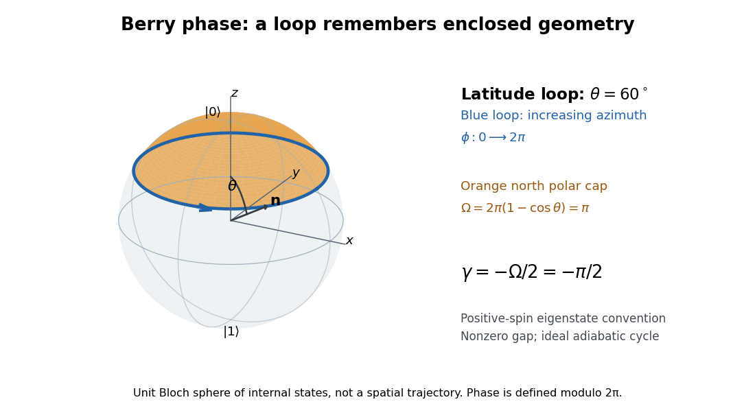
At , the solid angle is and the Berry phase is . At , the solid angle is and the Berry phase is . At , the loop collapses and . At , the same expression gives : the Bloch vector stays at the south pole, while this representative is . Its winding is only a choice of global phase, so the physically relevant phase factor is again one. The displayed formula is a continuous, unwrapped representative, not a unique real-valued observable.
For a normalized, smoothly chosen instantaneous energy eigenstate , the Berry connection has components . Its line integral around a closed parameter path gives the Berry phase in a periodic choice of state vector:Normalization makes the inner product purely imaginary, so the Berry connection is real. Changing the representative to changes the Berry connection to . A single-valued phase factor along the closed path changes the line integral by an integer multiple of , leaving unchanged. If the chosen vector is not periodic, include the endpoint phase:Here denotes the instantaneous energy eigenstate representative, with its dynamical phase removed. This is freedom to choose a representative of a state ray. [ref]
https://davidtong.org/pdfs/teaching/quantum-hall-effect/qhe1.pdf. David Tong, The Quantum Hall Effect, sections 1.5.1–1.5.2: Berry connection and a spin example; the spin convention below is stated explicitly
.The Euler evaluation of even zeta values turns a family of series into exact expressions using Bernoulli numbers, factorials and powers of . For every positive integer ,Here is the Riemann zeta function, defined by its convergent series at these arguments, and the Bernoulli number convention is . The alternating sign combines with the sign of to give a positive sum.[ref]
Substituting , and givesThe first identity answers the Basel problem. It is surprising because the original series only mentions reciprocal squares of integers, while its exact sum involves the circle constant . The cotangent partial-fraction expansion supplies a connection between the two: trigonometric functions encode equally spaced integer poles, whose expansion brings the reciprocal powers into view.
For an original numerical comparison, the first ten terms give , while . The omitted positive terms still contribute approximately . For fourth powers, the ten-term partial sum is approximately , only below . Both are convergent series, but the second approaches its limit much faster.
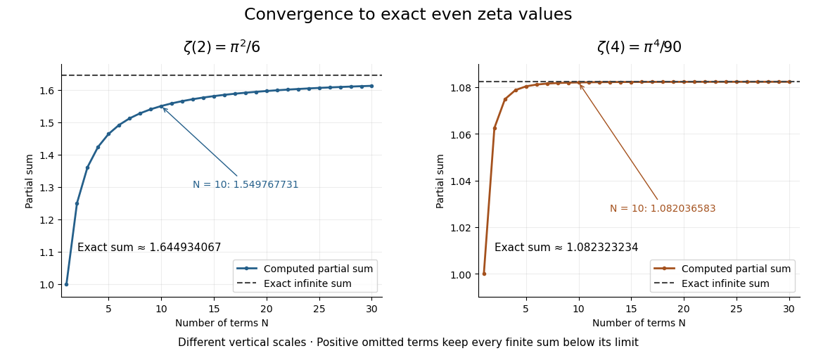
Exact evaluation is useful beyond obtaining more digits. It supplies an independent check on a numerical summation, exposes how Bernoulli numbers organize infinitely many identities, and makes the remaining series truncation error measurable without knowing any omitted terms individually. The even integer condition is essential to this formula: putting into it is not a way to evaluate , since the required Bernoulli number index and factorial expression here are indexed by positive integers.
Historically, Leonhard Euler announced reciprocal-square and reciprocal-fourth-power evaluations in §2 of On the sums of series of reciprocals by Leonhard Euler. That paper was presented on 5 December 1735 and published in 1740, as the English translation's first-page note records. His §§3–8 develop a route through the sine power series and relationships between roots and coefficients. The cotangent calculation below is a concise modern presentation of the connection.[ref]
On the sums of series of reciprocals by Leonhard Euler. English translation, p. 1, §2 and publication note; pp. 3–4, §§3–8: sine series, roots and coefficients
Hyperbolic cotangent generating function for Bernoulli numbers by Codex 0 Created 2026-10-13 Updated 2026-11-05
Codex 0 Created 2026-10-13 Updated 2026-11-05The defining generating function of the Bernoulli numbers, with , gives this identity of formal Laurent series by . Therefore is regular and odd. Integrating it gives the even formal logarithm of . Its even derivatives of order at zero are , while the odd derivatives vanish. This computes the cyclotomic higher logarithmic derivatives of symmetric cyclotomic units without introducing a spurious linear term.
The Bernoulli polynomials extend the Bernoulli numbers by inserting the exponential function into their exponential generating function:For example, , , , and .[ref]
NIST Digital Library of Mathematical Functions. Karl Dilcher, Chapter 24, equations 24.2.3–24.2.5 and Table 24.2.2
Their crucial property is a finite difference identity:Indeed, subtracting the two exponential generating functions cancels and leaves . Thus plays for discrete summation the role that plays for integration: taking a unit finite difference recovers .[ref]
Local flag correction of a Bell-state phase mixture by Codex 0 Created 2026-10-13 Updated 2026-10-20
Codex 0 Created 2026-10-13 Updated 2026-10-20Suppose Alice holds a classical orthogonal flag for the phase of a Bell state:Her local controlled phase correction maps this to . Thus Alice and Bob recover an exact Bell pair without revealing its bit value. Even if Eve knows the flag, purity decouples a subsystem from its purification, so the corrected pair can supply a private bit. Discarding the flag first can instead yield a separable quantum state, as happens at .
Base pairing is the recognition and association of compatible nucleobases. In canonical Watson–Crick geometry, an adenine–thymine base pair has two hydrogen bonds, while a guanine–cytosine base pair has three. These counts refer to those specific geometries and usual chemical forms; they are not a definition of every possible base pair. RNA can also contain other pairings, and canonical adenine–uracil pairing replaces adenine–thymine pairing. See Clark, Douglas and Choi, Biology 2e: DNA structure.
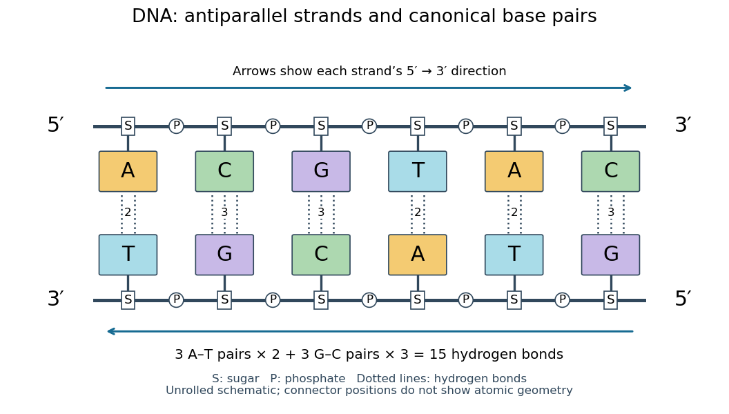
Six canonical Watson–Crick DNA base pairs: opposite backbone directions and two or three hydrogen bonds per pair
. Details. For this illustrative duplex, the six base pairs are A–T, C–G, G–C, T–A, A–T, and C–G. Thus three contribute two hydrogen bonds each and three contribute three each:Each dotted connector in the diagram counts one hydrogen bond; coloured boxes denote whole nucleobases, not individual chemical atoms. The solid rails denote the covalent bond scaffold. Separating the two strands disrupts base pairing and base stacking without requiring the backbone to be cut.
The count of fifteen hydrogen bonds is not fifteen identical contributions to a duplex's Gibbs free energy. Base stacking, interactions with water and ions, temperature, and the order of neighbouring base pairs also matter. Knowing the fraction of guanine–cytosine base pairs alone does not fix a nucleic acid double helix's shape or stability. See Brown, Genomes: pairing and stacking interactions. What makes base pairing especially useful is its selectivity: an exposed DNA strand constrains the partner's nucleic acid sequence, giving DNA replication a chemical recognition rule.
The cosmological baryon density is the mass density in baryonic matter, including hydrogen and helium. Up to nuclear binding-energy and composition corrections it is the proton mass times the baryon number density. The baryon-to-photon ratio links that number density to the photon number density. Larger baryon density increases nuclear reaction rates and permits the deuterium bottleneck to end earlier.
Pinned article: Introduction to the OurBigBook Project
Welcome to the OurBigBook Project! Our goal is to create the perfect publishing platform for STEM subjects, and get university-level students to write the best free STEM tutorials ever.
Everyone is welcome to create an account and play with the site: ourbigbook.com/go/register. We belive that students themselves can write amazing tutorials, but teachers are welcome too. You can write about anything you want, it doesn't have to be STEM or even educational. Silly test content is very welcome and you won't be penalized in any way. Just keep it legal!
Intro to OurBigBook
. Source. We have two killer features:
- topics: topics group articles by different users with the same title, e.g. here is the topic for the "Fundamental Theorem of Calculus" ourbigbook.com/go/topic/fundamental-theorem-of-calculusArticles of different users are sorted by upvote within each article page. This feature is a bit like:
- a Wikipedia where each user can have their own version of each article
- a Q&A website like Stack Overflow, where multiple people can give their views on a given topic, and the best ones are sorted by upvote. Except you don't need to wait for someone to ask first, and any topic goes, no matter how narrow or broad
This feature makes it possible for readers to find better explanations of any topic created by other writers. And it allows writers to create an explanation in a place that readers might actually find it.
Figure 1. Screenshot of the "Derivative" topic page. View it live at: ourbigbook.com/go/topic/derivativeVideo 2. OurBigBook Web topics demo. Source. - local editing: you can store all your personal knowledge base content locally in a plaintext markup format that can be edited locally and published either:This way you can be sure that even if OurBigBook.com were to go down one day (which we have no plans to do as it is quite cheap to host!), your content will still be perfectly readable as a static site.
- to OurBigBook.com to get awesome multi-user features like topics and likes
- as HTML files to a static website, which you can host yourself for free on many external providers like GitHub Pages, and remain in full control

Figure 2. You can publish local OurBigBook lightweight markup files to either OurBigBook.com or as a static website.
Figure 3. Visual Studio Code extension installation.
Figure 5. . You can also edit articles on the Web editor without installing anything locally. Video 3. Edit locally and publish demo. Source. This shows editing OurBigBook Markup and publishing it using the Visual Studio Code extension. 
- Infinitely deep tables of contents:




All our software is open source and hosted at: github.com/ourbigbook/ourbigbook
Further documentation can be found at: docs.ourbigbook.com
Feel free to reach our to us for any help or suggestions: docs.ourbigbook.com/#contact