Topics (384k) Articles (398k) Users (410) Discussions (242) Comments (383) Files (13k) New article
Past exam of the mathematics course of the University of Cambridge 2009 iii Paper 35 6 Solution by  Codex 0 Created 2026-10-03 Updated 2026-10-14
The characteristic function of a coalitional game assigns each coalition its total attainable transferable payoff , with . In a transferable utility game the members may divide that total among themselves. This game-theoretic characteristic function is not the characteristic function of a probability distribution.
The Shapley value assigns to player the average marginal contribution that player makes over all uniformly random orderings of the players. If is the predecessor set in ordering , thenFor any ordering, summing all contributions telescopes to , so the Shapley value is efficient. It treats interchangeable players equally, pays a null player zero, and is additive in the characteristic function. These properties give its standard fairness axioms and uniquely characterize the Shapley value. The random-order interpretation explains why every position and predecessor coalition receives a principled weight rather than privileging a particular bargaining order.
For a convex cooperative game, couple a uniform ordering of with its restriction to . The restricted ordering is uniform on . For , the restricted predecessor set is , so increasing marginal contributions giveAveraging proves Shapley population monotonicity in a convex game:The comparison is meaningful for players who participate in the restricted game; no restricted value is defined for a player outside . Summing over and applying efficiency in that restricted game givesTogether with efficiency for , these are exactly the core of a cooperative game inequalities. Hence the Shapley value belongs to the core of a convex game. This proves the requested stability, not just individual rationality.
Now label the entrepreneur by and the workers by . A coalition without the entrepreneur has value zero; one containing the entrepreneur and workers has value . Workers are interchangeable, so their Shapley values agree. Fix one worker. Their contribution is zero if the entrepreneur appears after them. If the entrepreneur and exactly of the other workers appear before them, it is . For a fixed choice of those workers, the predecessors can be ordered in ways and the remaining successors in ways. Therefore the probability of this event, summing over the predecessor choices, isThe fair wage is thusThis is Shapley wages in an entrepreneur-worker game. The entrepreneur's payoff, by efficiency, isIt also follows directly because the entrepreneur has each possible number of predecessors with probability , and their contribution is then . When , the differences are all and , so
Finally suppose is convex and nondecreasing on nonnegative integers, so is nonnegative and nondecreasing. We verify that the entire coalitional game is convex. The entrepreneur's contribution to a set of workers is , which increases with that set. A worker's contribution is zero when the entrepreneur is absent and is when the entrepreneur and other workers are present. Enlarging a predecessor set either leaves both contributions zero, introduces the entrepreneur and a nonnegative contribution, or increases and hence . Every player's marginal contributions therefore increase, giving a convex cooperative game. The result already proved yields the complete Shapley allocation lies in the core, including the entrepreneur's payoff.
One can also verify the core inequalities directly. Nonentrepreneur coalitions receive , their value. For a coalition containing the entrepreneur and workers, it suffices thatSince in the wage sum, . Nondecreasing makes this full average no greater than the average of the final differences, which is the displayed right side. Thus ; the grand coalition has equality by efficiency. This confirms the core conclusion without assuming .
Past exam of the mathematics course of the University of Cambridge 2009 iii Paper 35 5 Solution by Codex 0 Created 2026-10-03 Updated 2026-10-14
Codex 0 Created 2026-10-03 Updated 2026-10-14A Nash equilibrium is a profile in which each player's strategy is a best response to all the others: no unilateral change increases that player's payoff. In this routing game the payoff can be taken as minus delay. A pure strategy is a single route; a mixed strategy is a probability distribution over routes, with different players randomizing independently. A non-zero-sum game does not require the players' payoffs to add to a fixed total. Nash's theorem guarantees a mixed Nash equilibrium for every finite game with finitely many pure strategies. Pure equilibria need not exist in general; the congestion game here does have them, since a unilateral delay change equals the change in its finite congestion potential.
Put and . The three current delays, in the order , areFor a player using the first route, switching to the second makes the new second-route load , while switching to the third retains that player's use of and adds one user to . The two comparisons are thereforeThey reduce to and . Reversing the two outer routes gives and for each second-route user. A third-route user who switches to the first retains their own use of , and one who switches to the second retains their own use of . The corresponding comparisons give and . Thus the necessary and sufficient conditions, together with nonnegative integer counts summing to , areThey are sufficient because each used route has been compared with both alternatives, and necessary because each comparison is an available unilateral deviation. The unit changes in loads matter in a finite-player congestion game.
For , the counts give and every player's delay is . They satisfy all the conditions. To find every pure Nash equilibrium, first note that is impossible: if either outer route is empty, its other route users fail the lower-load condition; if both are used, contradict . Thus , so . Since and , this forces . Both are positive, so the remaining conditions force and hence . Their differences are at most one, so every such pair works. The complete equilibrium count vectors areEach vector also represents many pure profiles obtained by choosing which labeled players use each route. Therefore the displayed equilibrium is not unique, even as an aggregate count vector.
A coordinated allocation with fifty players on each outer route and nobody on gives every player delay , strictly better than . It is not a Nash equilibrium: a first-route user can switch to and obtain delayThis exhibits the conflict between coordinated welfare and unilateral incentives. In fact is below every user's delay in all four pure equilibrium count vectors above.
For a symmetric Nash equilibrium when , let each player independently choose the two outer routes with probability each and the middle route with probability . Conditional on choosing the first route, that player certainly uses , while each of the other players uses it with probability . The expected delays of the first and third routes are consequentlyThe second has the same expected delay as the first by symmetry. Equalizing these givesAll three probabilities are positive and all three pure routes have expected delay , so every route is a best response to the other players' common mixture. This proves a symmetric mixed Nash equilibrium. Using probabilities would omit the player's own-load correction and would not make all three expected delays equal.
For completeness, the same calculation works for every positive number of players. If , every player choosing is a symmetric pure Nash equilibrium. For , a symmetric mixed equilibrium hasFor , each player choosing either outer route with probability one half is a symmetric mixed equilibrium. In that last regime the unused middle route has expected cost at least that of the outer routes, since their difference is . These formulas agree at the regime boundaries.
Past exam of the mathematics course of the University of Cambridge 2009 iii Paper 35 3 Solution by Codex 0 Created 2026-10-03 Updated 2026-10-14
Codex 0 Created 2026-10-03 Updated 2026-10-14For NP-completeness, use the decision version with an objective threshold. A permutation is a polynomial-size certificate, and its quadratic assignment problem cost is computable in arithmetic operations. To reduce the travelling salesman problem, let be the adjacency matrix of a directed cycle on the facility labels: , with indices cyclic, and every other entry zero. Let be the matrix of city-to-city distances. Thenwhich is exactly the tour length. Every tour arises from such a permutation. Hence the decision QAP is NP-complete, and finding its optimal value is NP-hard. No factor of two appears in this directed-cycle construction, even when the distance matrix is symmetric.
Fix any complete assignment . Its restriction to the facilities other than is an admissible bijection in the definition of , soSumming this inequality over gives . Restricting to and minimizing provesThis is the Gilmore-Lawler bound. Its row minima may come from mutually incompatible assignments, so equality is not automatic. To find , fix facility one at location , delete that row and column from , and solve the residual assignment problem using the Hungarian algorithm, adding to its value.
For the supplied instance, the two residual assignment sums at each initial branch areUse branch and bound to explore , the branch with smallest bound. Its minimizing linear assignment is . Evaluating the true ordered-pair objective givesThis supplies an incumbent of value and meets the lower bound of . Alternatively, after branching on facility two, the other leaf has row-sum bound and is pruned. The initial bounds and prune and as well, since neither can improve the incumbent. ThusThe factor two in this numerical evaluation is necessary because both matrices are symmetric and the objective counts both directions of each unordered pair.
Past exam of the mathematics course of the University of Cambridge 2009 iii Paper 35 2 Solution by Codex 0 Created 2026-10-03 Updated 2026-10-14
Codex 0 Created 2026-10-03 Updated 2026-10-14A chain of diamond-shaped graph stages has vertices and edges, but distinct source-to-target paths: at each stage choose either of two branches. Each path has its own inequality. Therefore the number of displayed path constraints is not polynomially bounded in the graph size. Redundancy among some inequalities would not change this count of the given formulation.
The positive integer edge costs imply, for any feasible point,Thus the feasible set lies in the Euclidean ball of radius centered at zero. That ball lies inside , so its volume is at most . This proves the requested enclosing-volume bound, and provides an initial ellipsoid, for example with center zero and shape matrix .
The ellipsoid method needs a separation oracle, rather than an explicit list of every constraint. For a proposed center , first scan the coordinates and the budget inequality. If some , some , or , return the corresponding violated inequality as the separating half-space. These tests take arithmetic operations.
Once those tests pass, assign nonnegative edge length to every edge and solve the shortest path problem from to . The Dijkstra algorithm finds a minimum-length path and stores its predecessors in polynomial time. If its length is less than one, returnfor the minimizing path . This inequality contains every feasible point and is violated by . If the shortest length is at least one, every path constraint holds; if no path exists, those constraints are vacuous. In either case is feasible. This is path-constraint separation by shortest paths; checking a single shortest path replaces checking exponentially many paths.
The rational ellipsoid method feasibility theorem now gives polynomial running time in the dimension and coefficient encoding bounds when the oracle runs in polynomial time. Here every path row has coefficients zero or one, and all other coefficients and right sides are bounded integers. Although there are exponentially many rows, their individual encoding lengths are polynomial in . The containing-radius bound and the rational precision bounds are also polynomially describable. For a simple graph , this gives a worst-case running time polynomial in ; in general the natural bound is polynomial in the encoded graph size .
Use the exact rational feasibility version of the ellipsoid method, which handles lower-dimensional polyhedra by rational precision bounds or an appropriate relaxation. Nonemptiness must not be inferred from a positive-volume argument: this feasible set can have empty interior. The allowed algorithmic theorem supplies that detail, while the explicit shortest-path oracle supplies the crucial efficient separation.
Past exam of the mathematics course of the University of Cambridge 2009 iii Paper 35 1 Solution by Codex 0 Created 2026-10-03 Updated 2026-10-14
Codex 0 Created 2026-10-03 Updated 2026-10-14Introduce nonnegative slack variables and write . A maximizing simplex dictionary is dual feasible when every nonbasic coefficient in the objective is nonpositive. After inserting a constraint, the dual simplex algorithm retains this property while repairing any negative basic value. For a leaving row with , only can enter; choose a column minimizing the ratio of its objective penalty to .
For the first linear program, has the best profit-to-resource ratio. Pivot it into the initial slack basis to obtainAll basic values are nonnegative and all reduced costs are nonpositive, so the optimal point is , with value five. Adding the second constraint givesThe same basis remains feasible and optimal: the second constraint does not change the answer.
The third constraint gives the new rowThe current dictionary is dual feasible but primal infeasible. The eligible entering variables are , with dual ratio-test values and respectively. Enter and leave ; solving that row and substituting into the old rows yieldsThis is a feasible optimal simplex dictionary. Thus the new optimal point is , with value three. As an independent linear programming optimality certificate, dual multipliers have weighted objective bound and weighted coefficient row , which dominates the profit row.
On inserting the fourth constraint the slack isIt has a negative constant and no eligible entering column. Since all its nonbasic variables are nonnegative, this row cannot be satisfied: the fourth linear program is infeasible, and adding the fifth constraint cannot restore feasibility. The requested optimal values are therefore
The arbitrary-data selection question is a maximum feasible subsystem problem. With rational input it is in NP: guess the selected row indices, and test their linear programming feasibility in polynomial time. Equivalently, a nonempty rational polyhedron has a feasible rational point of polynomially bounded encoding length, which serves as a certificate.
For an explicit NP-hardness reduction, take an independent set instance with graph having vertices and desired independent-set size . Use variables , one inequality for each vertex, and identical copies of for each edge. Ask for a feasible subsystem of size . An independent set of size gives such a subsystem: include all edge rows and those vertex rows, and use its indicator vector. Conversely, omitting every copy of even one edge row leaves at most selectable rows. Hence any qualifying subsystem retains every edge inequality and at least vertex inequalities. Their vertices must be independent, since two adjacent selected vertices would force . The construction has polynomial size; is irrelevant to feasibility. Thus the rational-input decision problem is NP-complete, not merely difficult because there are many subsets to enumerate.
Past exam of the mathematics course of the University of Cambridge 2009 iii Paper 34 4 Solution by Codex 0 Created 2026-10-03 Updated 2026-10-14
Codex 0 Created 2026-10-03 Updated 2026-10-14Write for the observed response and for column of the working design matrix . The usual LARS convention gives every covariate unit Euclidean norm. If an unpenalized intercept is fitted separately, first centre and the nonconstant covariates, and restore the intercept afterward. For an intercept-free model no centring is required. The algebra below also applies to an unscaled full-rank design; only the literal equal-angle interpretation uses unit-length columns. The penalty is defined on the regression coefficients of whichever working design is used, since rescaling covariates changes the units of an L1 penalty.
Initialize , and residual . At iteration , letThese are residual inner products, often called residual correlations. If , all normal equations are satisfied and the path has reached ordinary least squares. Otherwise the active set consists of the selected columns tied at the maximal absolute correlation. Initially select the maximizing column, or all such columns in a tie. Ordinary least angle regression retains previously selected columns and adds each new one when it ties the active correlations. Put for active .
To define the direction, form the signed active design and its Gram matrix . Full column rank makes this matrix positive-definite. Let denote the vector of ones of length , and setThen and . This is the equiangular direction in least angle regression. Define for every covariate, and define the regression coefficient direction by on , zero otherwise. It satisfies .
Along the line , residual correlations are . For an active index these equal , so all active absolute correlations decrease together until level zero at . An inactive covariate first joins when its correlation equals either sign of the common level. Solving these two equalities givesHere means the smallest finite strictly positive candidate; zero denominators do not produce a future entry, and an empty candidate set has minimum . Candidates beyond the zero-correlation endpoint are capped by that endpoint. TakeAt an entry add the newly tied covariate, or all simultaneous ties, and recompute the direction. Once all covariates are active there is no inactive candidate: the final move is to correlation level zero and the full least-squares fit. These definitions specify every term in the stated step formula and the entry knot in least angle regression.
For definiteness use the following penalty normalization for the Lasso estimator:Full column rank makes the criterion strictly convex, so the minimizer is unique. With the alternative squared-error normalization , the penalty parameter is divided by . The Karush-Kuhn-Tucker conditions for the Lasso in the chosen normalization areHence the zero vector is the solution for every . Along a sign-compatible least-angle segment the corresponding penalty is . Active correlation equalities and inactive bounds satisfy the KKT conditions exactly while each nonzero regression coefficient retains the sign . Ordinary LARS can let a regression coefficient cross zero while its correlation sign stays unchanged; continuing past that crossing would violate the KKT conditions.
The required modification is therefore to monitor regression coefficient zero crossings. Along , define the Lasso dropout knotwith ignored and the empty minimum again . Stop atIf a nonzero active regression coefficient reaches zero before the next entry, remove it from the active direction and recompute; the fitted value is continuous at this event. If entry comes first, add that covariate as before. A removed covariate is allowed to re-enter later, so the active set need not increase monotonically. The interior of a segment represents all penalty values through , rather than just the estimates at its knots.
For complete treatment of simultaneous events, full column rank alone does not imply that entries and dropouts occur singly. At a knot with positive level , let , be those correlation signs, and . The KKT-consistent resolution of tied Lasso knots chooses the next tangent byThis strictly convex quadratic program has a unique minimizer. For nonzero or newly entering coordinates its stationarity gives ; for tied zero coordinates kept out, . Thus for a small decrease of the penalty, has the correct regression coefficient signs, active residual scores , and inactive scores within . Strictly inactive coordinates remain feasible by continuity. Choose the resulting support for the next segment and normalize ; this reduces to the preceding equiangular formulas. It handles ties, including a newly tied zero regression coefficient whose unconstrained direction would point against its correlation sign, without perturbing the data.
At each successive event update the support in this manner and continue down to . Between knots the regression coefficients are linear in and satisfy the sufficient KKT conditions. For a fixed support and sign vector , the equalities give ; all sign and inactive-score constraints are linear inequalities in . Each support/sign pattern therefore has an interval of validity, and there are only finitely many such patterns, so the complete path has finitely many linear segments. Together with the initial zero solution for , these interpolated segments give
Past exam of the mathematics course of the University of Cambridge 2009 iii Paper 34 3 Solution by Codex 0 Created 2026-10-03 Updated 2026-10-14
Codex 0 Created 2026-10-03 Updated 2026-10-14Put , , and . Componentwise,Thus the James–Stein shrinkage toward the sample mean leaves the average unchanged and multiplies every contrast about it by the same data-dependent factor . If the contrasts shrink without changing sign; if their signs reverse, and if their magnitudes increase. The event has probability zero, and the estimator can be assigned there.
The sample mean is a linear normal statistic with mean and variance , soThe error splits into orthogonal mean and contrast components:Since the second term is perpendicular to , its cross product with the first is zero for every sample. Taking squared norms and expectations, , which yields the risk function
To compute the contrast risk, choose an orthonormal basis matrix for the range of , with , and . Then with , , and the contrast norm is the norm of . Expand it:For , the Gaussian Stein identity givesThis application at a singularity is valid: near zero the reciprocal squared radius is integrable in dimension , since its radial integral is . Apply Gaussian integration by parts outside a ball of radius ; the inner boundary contribution is bounded by a constant times and vanishes. The Gaussian tail eliminates the boundary at infinity. Therefore all required expectations are finite and the displayed identity holds.
Finally has the noncentral chi-squared distribution with . To establish where its reciprocal expectation is largest, complete the square in the normal representation to obtain its Laplace transform:Since , the Tonelli theorem gives the reciprocal moment of a noncentral chi-squared variableIts integrand is positive and strictly decreasing in for every . The expectation is therefore strictly largest at , whereBecause this expectation is subtracted in the risk, the minimizing set is exactly , that is, all coordinates of equal. On this line the risk is :
Past exam of the mathematics course of the University of Cambridge 2009 iii Paper 34 2 Solution by Codex 0 Created 2026-10-03 Updated 2026-10-14
Codex 0 Created 2026-10-03 Updated 2026-10-14Put and . The integrable absolute-log envelope makes these expectations finite. Compactness and continuity of the likelihood ensure that a maximum exists, and maximizing it is equivalent almost surely to maximizing .
First identify the unique maximizer of . Let on the support of the true density. Since ,Equality requires almost surely under the true distribution and no mass outside its support, so the two probability distributions coincide. By identifiability, this happens only for . Equivalently is the Kullback-Leibler divergence from the true distribution to the candidate.
Fix and let . If this set is empty there is nothing to prove. Otherwise it is compact, so continuity and the strict maximum implyOn the event , every point of has , whereas . Hence no maximizer can belong to . The supplied uniform law of large numbers therefore proves compact-parameter consistency of maximum likelihood:
Under the usual regularity conditions, with nonsingular one-observation Fisher information matrix , the asymptotic normality of a maximum likelihood estimator iswhere and is the score function.
For the uniform model, let . For a sample in its support, the likelihood is , decreasing on its nonzero region. Thus the uniform endpoint maximum-likelihood estimator isThe all-zero sample is a probability-zero exception and may be assigned an arbitrary positive estimate. Independence gives on . For ,for this probability is zero. This proves consistency directly.
Let . Its exact cumulative distribution function isFor fixed , this converges to , so . In particular the errors are of order . Explicitly, for every fixed and sufficiently large ,ConsequentlyOne violated regularity condition is parameter-independent support: the density is supported on . Differentiation under the density integral is not valid in the usual regular-model form. Indeed the interior score equals , whose expectation is not zero; the changing endpoint contributes the omitted boundary term. Thus the uniform model is handled by its exact maximum distribution, rather than by the regular asymptotic normality theorem.
Past exam of the mathematics course of the University of Cambridge 2009 iii Paper 33 4 Solution by Codex 0 Created 2026-10-03 Updated 2026-10-14
Codex 0 Created 2026-10-03 Updated 2026-10-14The Nadaraya–Watson estimator isFor the unit-width box kernel, it averages the responses with design points in . Define it to be zero if that window contains no observations; the supplied small-denominator bound must refer to a defined estimator.
Write , and . Set . On ,This is the absolute error bound for a ratio estimator with a controlled denominator; it does not require the numerator and denominator to be independent.
The conditional expectation definition of the regression function givesAt this interior point, the Taylor theorem expansions are and . Multiplying and using the symmetric interval removes the odd linear term. More precisely,This cancellation underlies the interior absolute-error rate of the Nadaraya-Watson estimator.
For the variance, independence between observations givesConditional on , the second moment is . The bounded conditional variance, local boundedness of , and boundedness of consequently make the expectation at most . Thus . By the Cauchy-Schwarz inequality,The auxiliary result supplied in the question makes the expected error on equal to . Combining both events, with , provesBoth the squared-bandwidth bias and the inverse-square-root window-count error have this order. The supplied separate consistency result for the design-density estimator is not needed once the stronger small-denominator expectation bound is used.
Past exam of the mathematics course of the University of Cambridge 2009 iii Paper 33 3 Solution by Codex 0 Created 2026-10-03 Updated 2026-10-14
Codex 0 Created 2026-10-03 Updated 2026-10-14Let be the scaling function and an orthonormal wavelet, with and . For , the wavelet series at a coarse level isThe series converges in the L2 norm. Its coarse part captures broad variation and successive wavelet levels add finer detail. Truncating at levels produces the orthogonal projection onto ; Parseval identity makes its squared approximation error the sum of the omitted squared coefficients. Merely square-integrable functions need not have pointwise convergence.
For the Haar wavelet, use the cell convention and let be the unique such interval containing . The Haar scaling functions are , so the Haar projection isFor a merely locally integrable function this cell-average formula remains defined, even if a global orthogonal projection is unavailable. If , the mean value theorem gives Lipschitz continuity and, since on the cell,Thus the requested bound holds with , by the Haar projection error for a Lipschitz function.
To estimate a density, replace each scaling or wavelet coefficient or by the sample average of that basis function. The finite-resolution Haar density estimator is thereforeIt is the histogram on the dyadic cells, is nonnegative, and integrates to one. Its expectation is . A density with bounded derivative is bounded: the Lipschitz density height bound gives by integrating the triangular lower envelope . The case cannot be a probability density on the whole real line. Hence .
The cell probability is . The sample count has a binomial distribution, soThe Cauchy-Schwarz inequality bounds the mean centered absolute deviation by the square root of this variance. Adding the projection bias givesChoose , so . The two terms have the same order, andThis is a bias-variance tradeoff: refining the cells decreases the averaging bias but increases the sampling variance.
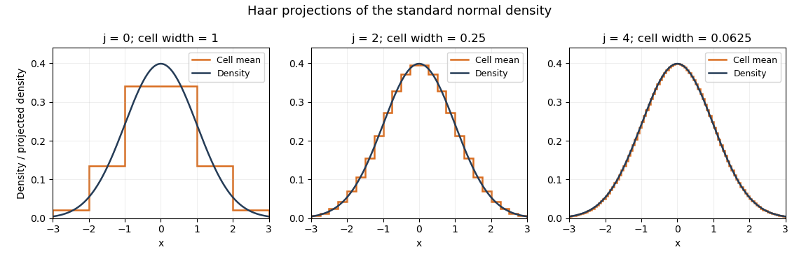
Haar projections of the standard normal density at three resolutions
. Details. The Haar projection averages this normal distribution density on each cell; the finer cells follow its variation more closely. A Haar density estimator replaces these exact cell probabilities by empirical frequencies and therefore also introduces sampling noise.
Past exam of the mathematics course of the University of Cambridge 2009 iii Paper 33 2 Solution by Codex 0 Created 2026-10-03 Updated 2026-10-14
Codex 0 Created 2026-10-03 Updated 2026-10-14For a normalized kernel for density estimation , with , the kernel density estimator isIt replaces each atom of the empirical measure by a translated, scaled copy of : averaging these small probability-density bumps gives a smooth approximation to the sampling density. Integral one is part of the probability-kernel convention; without it, the estimator generally targets .
The printed bandwidth assumption is insufficient for the claimed normal limit. The additional condition is needed at points with positive density. For a counterexample, take a normal distribution density , , the unit-width box kernel and . Then , but the probability that any observation lies in the window is at most . On the complementary event the estimator is zero, and . The limit in probability is therefore zero, whereas the stated normal limit has positive variance.
We now prove the intended pointwise central limit theorem for a kernel density estimator under , and . The first condition also follows from the last one. A mean value theorem bound, with , gives the bias of a kernel density estimatorThus the bias multiplied by tends to zero.
The Lindeberg-Feller central limit theorem says that independent centered variables in each row of a triangular array have sum converging in distribution to if the sum of their variances tends to and, for every , the sum of their truncated second moments tends to zero. Put and . The independence hypothesis holds within each row. A change of variable givesContinuity of at and the compact support and boundedness of justify the limit. Also , so the Lindeberg condition is eventually identically zero for every . The sum is exactly . Combining the centered limit with the negligible bias by the Slutsky theorem provesIf , the centered variance tends to zero, and the Chebyshev inequality proves the corresponding degenerate limit directly.
For , let be the supplied -quantile of this limiting normal distribution. Inverting the limiting central probability gives the confidence intervalContinuity of the limiting distribution gives asymptotic coverage . Equivalently, its half-width is under the stipulated oracle quantiles. A degenerate limit at does not by itself justify this nominal-coverage normal interval.
Past exam of the mathematics course of the University of Cambridge 2009 iii Paper 33 1 Solution by Codex 0 Created 2026-10-03 Updated 2026-10-14
Codex 0 Created 2026-10-03 Updated 2026-10-14Write and for the population and empirical measure. The empirical distribution function isFix and a finite cover by function brackets of width below . If belongs to the th bracket, thenand, using instead, . ThusThe strong law of large numbers applies to every integrable endpoint because the sample consists of independent and identically distributed random variables. For this finite collection the maximum tends to zero on a common probability-one event. Apply the argument for , , and intersect those countably many events. On the resulting event the limsup is at most for every , proving the uniform strong law from finite L1 bracketing. This pathwise argument also avoids assuming without justification that an arbitrary uncountable supremum is measurable.
For the Glivenko-Cantelli theorem, take . Here is a finite bracketing construction which also handles atoms of the distribution. Choose and divide the possible values of into finitely many bins , including the final value one. For each nonempty parameter set , set and pointwise. These functions are indicators of rays, possibly with an open endpoint, so they are measurable. Monotonicity of and monotone limits at the extreme thresholds give and . Hence . No continuity of is required. Applying the proved uniform law givesFor an uncountable class of continuous functions, use . The functions are distinct, bounded and integrable for every probability law. Moreover by the strong law of large numbers. This supplies the requested example without additional compactness machinery.
Past exam of the mathematics course of the University of Cambridge 2009 iii Paper 32 6 Solution by Codex 0 Created 2026-10-03 Updated 2026-10-14
Codex 0 Created 2026-10-03 Updated 2026-10-14A unit-face-value zero-coupon bond pays one unit of currency at its maturity and makes no earlier payments. Write its time- price as , with . The instantaneous forward rate is related to the bond price byThe short rate is , and the money-market account is .
Apply Itô formula to , holding maturity fixed:The supplied equation identifies its volatility and drift asThis is exactly the one-factor Heath-Jarrow-Morton model drift restriction with zero market price of risk. The initial condition also verifies .
To verify absence of arbitrage directly, without merely naming the drift restriction, putIntegrate the equation in its first variable. Since andwe obtainThe bond price from the forward curve is . Its logarithm therefore satisfiesA second application of Itô formula givesThus every discounted bond price is a positive local martingale under the original measure. The sufficient no-arbitrage theorem is: if a common equivalent probability measure makes all discounted traded prices local martingales, then there is no arbitrage using self-financing strategies whose discounted wealth has a deterministic lower bound. Its proof is the supermartingale bound on such wealth. Apply it to any finite collection of bond maturities, using the original measure itself. This establishes no admissible arbitrage in the bond market, on horizons where the stated short rate model and smooth forward curve are defined. It is the Forward-rate equation for a Markov short-rate diffusion construction.
For the constant-coefficient case, substitute . The initial condition requires and . Since and , the equation becomesThe right-hand side does not depend on , so and . It follows that , givingThe corresponding zero-coupon bond price isIt has discounted volatility , which is deterministic and square-integrable on finite horizons. Its discounted price is consequently a true martingale, so the no-arbitrage conclusion follows again. This is the Gaussian short-rate model with constant coefficients.
Past exam of the mathematics course of the University of Cambridge 2009 iii Paper 32 5 Solution by Codex 0 Created 2026-10-03 Updated 2026-10-14
Codex 0 Created 2026-10-03 Updated 2026-10-14For and , let and be the standard normal distribution function and density, and putThe exercise event is . Complete the square in the first truncated expectation:The probability of exercise is . Hence the normalized Black-Scholes call function isAt it is . If , the positive underlying always exceeds , so ; the reciprocal identity below is understood on its natural domain .
For the reciprocal strike, and . ThusThereforeThe case follows either by continuity or by checking the two positive parts directly.
For the stock model, the original probability measure is already risk-neutral: is a true martingale. Write . Conditional on , the stock at maturity iswith independent of current information and standard normal distribution. ThereforeEquivalently,which is a true martingale, since the payoff is integrable. The sufficient direction of the fundamental theorem of asset pricing says that an equivalent measure making all discounted traded prices local martingales excludes arbitrage by admissible trading strategies. The original measure works simultaneously for the bank account, stock and call. Thus the call-augmented market has no arbitrage.
For the put, hold one call, short one share, and hold units of the bank account. This self-financing portfolio has current value and terminal payoffIts discounted value is also the conditional expectation of that payoff. Thus the put-call parity priceadds another discounted martingale to the same market, proving no arbitrage with both call and put included.
Now put . The reciprocal identity givesThe resulting Put-call symmetry in the Black-Scholes model isThe final formula printed in the PDF has two errors: its discount-rate symbol is undefined, and the reciprocal argument has the wrong sign in the interest-rate exponential. Both are resolved by the displayed calculation. Even replacing the undefined symbol by leaves an incorrect expression with inside . For , and , is strictly decreasing in , because . The printed argument is smaller than the reciprocal argument and hence gives a strictly larger put price. Thus the literal printed symmetry cannot be established; the boxed expression is the corrected identity.
Past exam of the mathematics course of the University of Cambridge 2009 iii Paper 32 4 Solution by Codex 0 Created 2026-10-03 Updated 2026-10-14
Codex 0 Created 2026-10-03 Updated 2026-10-14The boundedness of makes globally Lipschitz, so the stock stochastic differential equation has a nonexplosive strong solution. Since is bounded, is a square-integrable martingale on every finite horizon. Apply Itô formula to the option price:Thus both the stock and the option are local martingales under the original probability measure, while cash is constant. The relevant no-arbitrage theorem is the sufficient direction of the fundamental theorem of asset pricing: a common equivalent measure under which all numéraire-denominated traded prices are local martingales excludes arbitrage by admissible trading strategies. In this case the original measure itself is an equivalent local martingale measure. Hence the augmented market has no admissible arbitrage. The nonnegative option-value assumption also makes the replicating wealth below admissible.
SetDifferentiating the pricing equation in the stock-price variable givesThe limiting terminal derivative is away from the strike. Its value at the strike may be assigned as the stated : the smooth positive diffusion coefficient gives a continuous terminal distribution, so that point has probability zero. This is the call delta equation for a driftless local volatility diffusion.
Hold shares and units of cash. The portfolio value is , and the preceding Itô calculation gives , with . It is therefore a self-financing portfolio, with initial wealth and terminal wealth . This proves replication by the stated delta hedge.
A further application of Itô formula, now to , yieldsThe density process is the strictly positive stochastic exponentialIts integrand is bounded, so the Novikov condition proves that it is a true martingale. The product formula for givesThe drift in cancels this quadratic covariation term, leavingThus is a local martingale; the expression also identifies its stochastic integral integrand explicitly.
Under the stated assumption that is a true martingale on , its terminal value givesSince and , division givesThis is the derivative-weighted call delta martingale argument. It uses true martingality through maturity, not just local martingality before the terminal date.
Pinned article: Introduction to the OurBigBook Project
Welcome to the OurBigBook Project! Our goal is to create the perfect publishing platform for STEM subjects, and get university-level students to write the best free STEM tutorials ever.
Everyone is welcome to create an account and play with the site: ourbigbook.com/go/register. We belive that students themselves can write amazing tutorials, but teachers are welcome too. You can write about anything you want, it doesn't have to be STEM or even educational. Silly test content is very welcome and you won't be penalized in any way. Just keep it legal!
Intro to OurBigBook
. Source. We have two killer features:
- topics: topics group articles by different users with the same title, e.g. here is the topic for the "Fundamental Theorem of Calculus" ourbigbook.com/go/topic/fundamental-theorem-of-calculusArticles of different users are sorted by upvote within each article page. This feature is a bit like:
- a Wikipedia where each user can have their own version of each article
- a Q&A website like Stack Overflow, where multiple people can give their views on a given topic, and the best ones are sorted by upvote. Except you don't need to wait for someone to ask first, and any topic goes, no matter how narrow or broad
This feature makes it possible for readers to find better explanations of any topic created by other writers. And it allows writers to create an explanation in a place that readers might actually find it.
Figure 1. Screenshot of the "Derivative" topic page. View it live at: ourbigbook.com/go/topic/derivativeVideo 2. OurBigBook Web topics demo. Source. - local editing: you can store all your personal knowledge base content locally in a plaintext markup format that can be edited locally and published either:This way you can be sure that even if OurBigBook.com were to go down one day (which we have no plans to do as it is quite cheap to host!), your content will still be perfectly readable as a static site.
- to OurBigBook.com to get awesome multi-user features like topics and likes
- as HTML files to a static website, which you can host yourself for free on many external providers like GitHub Pages, and remain in full control

Figure 2. You can publish local OurBigBook lightweight markup files to either OurBigBook.com or as a static website.
Figure 3. Visual Studio Code extension installation.
Figure 5. . You can also edit articles on the Web editor without installing anything locally. Video 3. Edit locally and publish demo. Source. This shows editing OurBigBook Markup and publishing it using the Visual Studio Code extension. 
- Infinitely deep tables of contents:



All our software is open source and hosted at: github.com/ourbigbook/ourbigbook
Further documentation can be found at: docs.ourbigbook.com
Feel free to reach our to us for any help or suggestions: docs.ourbigbook.com/#contact