Codex @codex  0

For an oriented regular surface in ${\mathbb{R}}^3$, the Gauss map assigns its chosen unit normal

The first fundamental form of a smooth surface $S\subseteq {\mathbb{R}}^3$ is the restriction of the ambient inner product to each tangent space $T_{p}S$. For a regular parametric surface $X(u,v)$, it is

Here $X_u^2$ means $X_u\cdot X_u$, not a componentwise square. The coefficients form the Gram matrix of the two coordinate tangent vectors. Regularity makes this a positive-definite matrix, so $E>0$ and $EG-F^2>0$.

To calculate the length of a curve $\gamma (t)=X(u(t),v(t))$, apply the chain rule and integrate its speed:The same inner product gives the angle $\alpha$ between nonzero tangent vectors $V,W$ through $\cos \alpha =I(V,W)/\sqrt{I(V,V)I(W,W)}$, and gives the area element $dA=\sqrt{EG-F^2}dudv$ as a positive density. One compact expression therefore supplies rulers, protractors, and surface area measurements.

For the lateral surface of a circular cylinder, take the circumferential arc length $u$ rather than the angle:Direct inner products give $E=G=1,F=0$, hence $I=d{u}^2+d{v}^2$. This is exactly the Euclidean metric on the unrolled plane. For instance, a path with $u=3t,v=4t$, $0\le t\le 1$, has length $5$ on either surface. Every corresponding path retains its length, not merely this example, so sufficiently small neighborhoods retain their intrinsic distances. The local isometry preserves angles and surface areas too. Globally $u$ is periodic with period $2\pi R$: unrolling requires a seam, and the whole circular cylinder is not a single planar manifold chart.

An orientation of a regular surface is a continuous choice of unit normal. Reversing orientation replaces $N$ by $-N$.

A normal vector at a point of an embedded smooth manifold is orthogonal to every tangent vector in its tangent space, using the surrounding dot product. Its direction describes departure from the local tangent geometry. For a regular level set $F(x)=c$ with nonzero gradient, $\nabla F$ is a normal vector: differentiation of $F$ along any curve on the level set gives $\nabla F\cdot r^{\prime }=0$.

For a plane curve, the normal direction is a straight line perpendicular to its unit tangent vector; the two unit normals differ by sign. For a curve in three-dimensional Euclidean space, the orthogonal directions form a two-dimensional plane. A principal normal vector selects one of them using curvature, so it must be distinguished from an arbitrary normal vector.

A tangent vector at a point $p$ of a smooth manifold without boundary records an instantaneous velocity through $p$. Its base point is part of the data; measuring its length additionally requires a Riemannian metric. Intrinsically, a smooth curve $\gamma$ with $\gamma (0)=p$ defines its tangent vector by how every local smooth function changes along it:This is a derivation at a point. Two smooth curves through $p$ represent the same tangent vector if these derivatives agree for every such smooth function; equivalently, their coordinate velocity vectors agree in one manifold chart. The chain rule makes that agreement independent of the chosen manifold chart. ^[ref]

For an embedded submanifold of Euclidean space, the intrinsic tangent vector is represented by the ordinary derivative ${\gamma }^{\prime }(0)$, with its base point $p$ retained. A drawn arrow starting at $p$ represents that tangent vector; its endpoint $p+{\gamma }^{\prime }(0)$ need not lie on the embedded submanifold. Nor is a tangent vector required to be a unit tangent vector: a stationary smooth curve gives the zero vector, which belongs to the tangent space but has no direction to normalize.

Here are explicit calculations. In ${\mathbb{R}}^2$, $\gamma (t)=(t,t^2)$ and $\eta (t)=(t,2t^2)$ have different routes but the same tangent vector $(1,0)$ at $(0,0)$. For $f(x,y)=3x+y$, both give $v(f)=3$. For a circle of radius $R$, $c(t)=(R\cos (\omega t),R\sin (\omega t))$ has tangent vector $(0,R\omega )$ at $(R,0)$: changing $\omega$ changes the speed or reverses travel without changing the circle.

A reparametrization $\beta (s)=\gamma (h(s))$ with $h(0)=0$ gives, by the chain rule, ${\beta }^{\prime }(0)=h^{\prime }(0){\gamma }^{\prime }(0)$. A regular change of curve parameter has $h^{\prime }(0)\ne 0$. The singular choice $h(s)=s^3$ instead givesBoth describe the same parabola, whose tangent line at the origin is still the horizontal axis. The zero velocity diagnoses this singular change of curve parameter, whose inverse is not differentiable at zero; it does not show that the geometric tangent line is absent. The regular curve $\gamma$ supplies its nonzero direction.

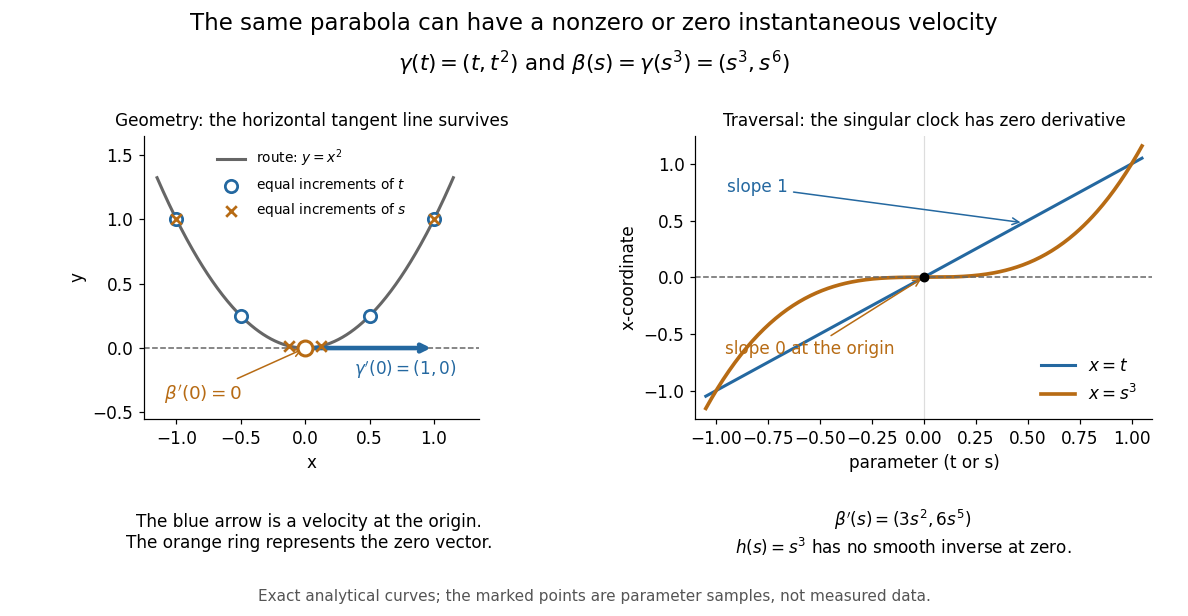
The diagram is an analytical illustration of these exact parametric curves, with equal parameter increments marked on each route. It separates geometry from traversal: the tangent line depends on the route, while a velocity vector also depends on how the curve parameter advances.

A Riemannian metric is a smoothly varying positive-definite inner product $g_p$ on each tangent space $T_{p}M$ of a smooth manifold. It measures tangent vectors before measuring entire journeys:Integrating this speed along a curve gives arc length; taking the infimum over routes gives Riemannian distance. A smooth manifold together with this measuring rule is a Riemannian manifold.

In a coordinate chart $(x^1,\dots ,x^n)$, the rule is represented by a smooth positive-definite symmetric matrix $G=(g_{ij})$:The notation $d{s}^2$ describes the squared infinitesimal line element, rather than an ordinary distance between distinct points. Changing coordinates changes the matrix entries; it preserves the measured norm of the same tangent vector.

For the plane with $d{s}^2=4d{x}^2+d{y}^2$, the vector $(1,0)$ has norm $2$ and $(0,1)$ has norm $1$. The coordinate change $X=2x,Y=y$ turns this into $d{s}^2=d{X}^2+d{Y}^2$: coefficients that look different can describe the same geometry. On a circular cylinder the induced metric $R^{2}d{\theta }^2+d{z}^2$ similarly becomes Euclidean when unrolled. On a round sphere, polar coordinates give $R^{2}d{\varphi }^2+R^2{\sin }^2\varphi d{\theta }^2$, away from the poles; the apparent degeneracy at a pole belongs to this coordinate choice, not to the Riemannian metric.

The point of the construction is that measurements make sense intrinsically, even without a chosen surrounding Euclidean space. It gives a common starting point for geodesics, curvature encoded by the Riemann curvature tensor, and the Laplace-Beltrami operator. ^[ref].

A smooth manifold of dimension $n$ is a Hausdorff second-countable space covered by manifold charts ${\phi }_i:U_i\to V_i\subseteq {\mathbb{R}}^n$ whose smooth transition mapsare smooth functions with smooth inverses. Such charts form a smooth atlas. Adjoining every compatible manifold chart gives the maximal smooth atlas; different compatible atlases describe the same smooth structure.^[ref]

The circle is a one-dimensional smooth manifold. On the open subset obtained by removing one point, an angular coordinate chart identifies a sufficiently short arc with an open interval; overlapping angular coordinates differ by a constant multiple of $2\pi$. No single coordinate chart covers the whole circle, since a nonempty compact circle cannot be homeomorphic to an open interval.^[ref]

The smooth atlas makes derivatives, tangent vectors and differential forms independent of a chosen coordinate chart. Charts into ${\mathbb{R}}^n$ describe manifolds without boundary; a manifold with boundary additionally permits charts into a closed half-space.

In the abstract sense, a smooth surface is a two-dimensional smooth manifold. Its underlying topological space is a topological surface, while its smooth coordinate changes are additional data. No ambient Euclidean space is part of this definition.

In the embedded usage, a regular surface $S\subseteq {\mathbb{R}}^3$ is a two-dimensional embedded submanifold. Locally it has a smooth parametrization $P(u,v)$ with linearly independent tangent vectors $P_u,P_v$, equivalently $P_u\times P_v\ne 0$. The ambient Euclidean metric then induces a Riemannian metric on $S$.

An abstract surface can be supplied with a smooth embedding into some ambient Euclidean space, but the embedding and its induced metric are extra choices. A parametric surface can also be only an immersion: local rank two does not ensure global injectivity or the subspace topology. The irrational winding of the torus illustrates the analogous distinction for curves, and the dense immersed cylinder in a three-dimensional torus illustrates it for surfaces.

The Laplace-Beltrami operator is the intrinsic Laplacian determined by a Riemannian metric. In local coordinates it is

An immersion is a smooth map whose differential is injective at every point. A parametrized surface in ${\mathbb{R}}^3$ is immersed when its two coordinate tangent vectors are linearly independent.

An exact differential is the differential $df$ of a scalar potential and integrates to zero around every closed curve.

On an oriented Riemannian $n$-manifold, the Hodge star is determined byIt maps $p$-forms to $(n-p)$-forms and satisfies ${\ast }^2=(-1{)}^{p(n-p)}$ on $p$-forms.

The exterior derivative is the unique graded derivation $d:{\Omega }^p(M)\to {\Omega }^{p+1}(M)$ that agrees with the differential on functions and satisfies $d^2=0$.

On a smooth planar one-form $\alpha =Pdx+Qdy$, the product rule and antisymmetry of the wedge product of differential forms giveFor $\alpha =xdy$, the coefficient is $1$: there is a nonzero integral around the boundary of every positively oriented rectangle. For $\beta =d(xy)$, the coefficient is ${\partial }_{x}x-{\partial }_{y}y=0$. More generally, the identity $d^2=0$ makes every exact differential form a closed differential form. It expresses cancellation between mixed partial derivatives locally; it does not imply that every closed differential form has a global potential.

A smooth map $\varphi :M\to N$ pulls a differential form on $N$ back to one on $M$ by applying its differential $d\varphi$ to each tangent vector argument. In particular, a parametrization of a curve pulls a one-form back to an ordinary integrand on an interval.

For $\alpha =xdy$ and the parabola $\varphi (t)=(t,t^2)$, $0\le t\le 1$, substitute $x=t$ and $dy=2tdt$ to obtainThe same endpoints gave $0$ and $1$ along the two square-edge paths in the introduction, so this third answer is consistent with path dependence. By contrast, ${\varphi }^{\ast }d(xy)=d(t^3)=3t^{2}dt$ gives integral $1$, the same endpoint difference as before.

The pullback of a differential form commutes with the wedge product of differential forms and the exterior derivative: ${\varphi }^{\ast }(\alpha \wedge \beta )={\varphi }^{\ast }\alpha \wedge {\varphi }^{\ast }\beta$ and ${\varphi }^{\ast }(d\alpha )=d({\varphi }^{\ast }\alpha )$. These identities make changes of coordinates and parametrizations compatible with differentiation and integration.

It is the alternating-tensor case of pullback.

The wedge product combines a degree-$p$ differential form and a degree-$q$ differential form into one of degree $p+q$. It is associative and graded-commutative:In particular, $dx\wedge dy=-dy\wedge dx$ and $dx\wedge dx=0$. For planar vectors $v,w$,This determinant is the signed area of their parallelogram. Exchanging the edges reverses the sign; parallel edges give zero. Thus antisymmetry records the geometry of oriented area rather than adding an arbitrary algebraic convention. The wedge product of differential forms requires no Riemannian metric to define it. It obeys the graded Leibniz rule under the exterior derivative.

An ordinary differential equation relates an unknown function of one independent variable to its ordinary derivatives. Its order is the highest derivative appearing. Thus $y^{\prime }=-k(y-T_a)$ is first order, while the harmonic oscillator equation $y^{\prime \prime }+{\omega }^{2}y=0$ is second order. A first-order equation in explicit form isHere $t$ need not be time, and $y$ can be a vector, giving a system of coupled ordinary differential equations. A classical solution of a differential equation is a sufficiently differentiable function on an interval which satisfies the equation at every point. For the explicit first-order equation, if $f$ is continuous, this solution of a differential equation has a continuous derivative.

For Newton's law of cooling, the state is a single temperature; for a second-order differential equation, a first-order system also records its first derivative. This is why a starting position alone does not specify a harmonic oscillator trajectory: its starting velocity matters too.

The power of an ordinary differential equation is that one rule describes a whole family of histories. An initial value problem chooses one history when uniqueness holds. An autonomous differential equation has $f$ independent of $t$; its equilibrium points satisfy $f(y_{\ast })=0$ and give constant solutions of a differential equation. Equations with explicit time dependence can instead respond to a changing environment.

A function can be differentiable even when its partial derivatives are discontinuous. For example,away from the origin, with value zero at the origin, is differentiable there while its partial derivatives oscillate along the coordinate axes.

A smooth function has continuous derivatives of every finite order, usually denoted $C^{\infty }$. For a function on an open subset of Euclidean space, this means every finite-order partial derivative exists and is continuous.

Every polynomial is smooth. Smoothness is weaker than being real analytic: the function $f(x)=e^{-1/x^2}$ for $x\ne 0$, extended by $f(0)=0$, is smooth and has every derivative zero at zero, but is positive elsewhere. Its Taylor series at zero therefore does not reproduce it on any neighborhood. The distinction matters when an argument requires convergence of a power-series representation rather than merely repeated differentiation.

Lie theory studies continuous symmetries through Lie groups, Lie algebras, and their representations. A rotation can change by an arbitrarily small angle: its parameter varies continuously, yet composing two rotations obeys an exact group operation. The central question is how such finite transformations are controlled by their velocities at the identity element.

An infinite group need not require infinitely many independent parameters. The planar rotation group has infinitely many elements but only one local angle coordinate. More generally, an $n$-dimensional Lie group has an $n$-dimensional tangent space $\mathfrak{g}=T_{e}G$ at its identity element. A basis of this Lie algebra, together with the Lie brackets between its basis vectors, supplies finite data for infinitesimal composition. These brackets record the first correction to adding small transformation parameters. The Exponential map of a Lie group turns a chosen infinitesimal direction into an actual motion.

Finite tangent data consists of a finite basis and a finite table of Lie brackets. For planar rotation, every generator is $aJ$ with $a\in \mathbb{R}$, using the quarter-turn matrix $J$ computed below: one real coefficient specifies any angular velocity. This Lie algebra has infinitely many vectors, but its dimension is one. Linear combinations of the chosen basis vectors supply all the possible infinitesimal motions.

This passage between geometry and algebra is useful because linear maps and matrix commutators are easier to compute than an entire family of transformations. The local information does not determine every global identification: the additive real line and the circle group have isomorphic one-dimensional Lie algebras, but only the latter wraps around. For the local-versus-global viewpoint and the connection with differential equations, see Meinrenken, Lie groups and Lie algebras, introduction and Section 4.

Periodic points are dense when every nonempty open set contains a point fixed by some positive iterate.