
Past exam of the physics B course of the University of Cambridge 2017 Paper 2 Section C C10 Solution 2026-10-18
A Carnot cycle consists of four reversible stages: isothermal expansion at the hot-reservoir temperature , adiabatic expansion to , isothermal compression at , and adiabatic compression back to the starting state. The adiabatic stages exchange no heat. For one mole of an ideal gas, the two isothermal stages have heats and in magnitude. The reversible adiabatic relations ensure .
More generally, the total entropy change over any reversible cycle is zero. The two heat exchanges therefore satisfyWith work output , its thermal efficiency isThe temperatures must be absolute. The second law makes this the maximum efficiency for an engine exchanging heat only with those two reservoirs; irreversible entropy production lowers the efficiency.
Past exam of the physics B course of the University of Cambridge 2017 Paper 2 Section B B9 Solution 2026-10-18
Following the moving fluid. The Eulerian velocity field assigns a velocity to each position. A fluid particle satisfies , so the chain rule gives the material derivative, also called the convective derivative,Even in steady flow a particle can accelerate because it moves between regions with different velocity. For example, flow around a curved obstacle changes direction despite . Mass conservation isFor a constant-density incompressible fluid, .
Euler equations for an inviscid fluid and Bernoulli's equation. Neglect viscosity and take the body force per unit mass to be . Newton's second law for a fluid element givesFor steady flow, dot with displacement along a streamline. The tangential component of is the derivative of along that line. For constant density, integration givesIn uniform gravity, . Thus pressure, kinetic energy per unit mass and gravitational potential energy per unit mass exchange along a streamline. For a barotropic compressible fluid, replace by . Different streamlines need not have the same Bernoulli constant.
Vorticity and potential flow. Vorticity is . A small fluid element rotates locally with angular velocity after its deformational part is separated. The vector identitygives for steady constant-density inviscid flow. Thus an irrotational region has one common Bernoulli constant on each connected region. In a simply connected irrotational domain, introduce a velocity potential . Incompressibility then gives Laplace's equation, . For unsteady irrotational flow,An impermeable stationary wall fixes , but ideal potential flow does not enforce no slip. In a multiply connected domain, irrotational flow may still have nonzero circulation around an excluded vortex core, so a globally single-valued potential requires care.
For example, uniform two-dimensional flow past a circular cylinder has outside . Its normal velocity vanishes at the cylinder, and its surface tangential velocity is . Bernoulli's equation predicts a symmetric pressure distribution and zero drag. This is D'Alembert's paradox: the assumptions omit the viscous boundary layers, separation and wake responsible for real drag.
For an incompressible fluid of constant kinematic viscosity , the curl of the motion equation givesThe first term stretches and tilts vortex lines; the second diffuses vorticity. In two-dimensional incompressible inviscid flow the stretching term is absent and vorticity is carried with the fluid. In a three-dimensional inviscid flow it can be amplified by stretching. Density gradients not parallel to pressure gradients provide an additional source in a general compressible fluid.
Viscous flow. A Newtonian fluid's shear stress is proportional to rate of strain. For constant viscosity and incompressibility the Navier-Stokes equation iswith dynamic viscosity and kinematic viscosity . At an ordinary solid wall, the no-slip boundary condition sets fluid velocity equal to the wall velocity. Viscosity transfers momentum between neighbouring layers and converts mechanical energy into heat; unlike the pressure force, its shear contribution depends on velocity gradients.
For plane Couette flow between plates , with the upper plate moving at , the steady solution is , with shear stress . For pressure-driven flow through a pipe of radius , a constant pressure gradient gives the parabolic Poiseuille profileThe Reynolds number compares convective inertia with viscous force. Small Reynolds number often permits the Stokes-flow approximation; large Reynolds number can produce thin boundary layers and, under suitable conditions, turbulence. It does not justify neglecting the wall conditions. Bernoulli's inviscid constant is generally not conserved along a viscous streamline, and pipe flow instead shows a pressure loss corresponding to dissipation.
Past exam of the physics B course of the University of Cambridge 2017 Paper 2 Section B B7 Solution 2026-10-18
Distributed circuit model. A transmission line must be treated as a distributed system when its propagation time is appreciable compared with the signal timescale. Divide a uniform two-conductor line into elements of length . Each has series resistance and inductance , and shunt electrical conductance and capacitance . The primes denote quantities per unit length, with units , , and , respectively.
Kirchhoff's voltage and current laws give the Telegrapher's equations:For a lossless line, , differentiation gives and the same wave equation for . The propagation speed and characteristic impedance areA general lossless signal has and . Thus characteristic impedance is the voltage/current ratio of one travelling wave, not simply the resistance of the wires. It can be real even when the line dissipates no energy, because energy is carried away by propagation.
For sinusoidal quantities with convention , the general lossy-line formulas areChoose the square-root branches for forward attenuation and positive forward power. The real part of is attenuation per unit length; its imaginary part is the phase wavenumber. For small losses, attenuation is approximately , using the lossless real in this estimate.
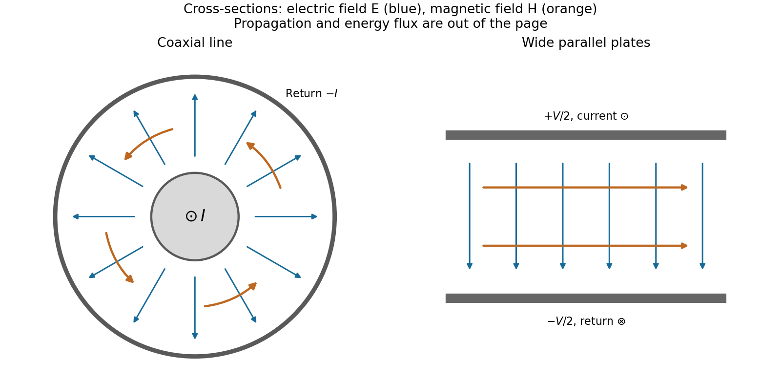
Fields and geometry. Two separated conductors support a transverse electromagnetic mode, with electric and magnetic fields transverse to the propagation axis. For a homogeneous dielectric and negligible conductor penetration, both examples below have and hence . The distributed circuit model follows from the field energy and charges in each slice.
For a coaxial cable with inner radius and inner surface of the outer conductor at , Gauss's law and Ampère's law giveThe electric field is radial and the magnetic field circles the axis. Integration of voltage and field energy givesThe equal and opposite return current on the outer conductor confines the ideal external field to the annulus.
For wide parallel plates of width separated by , neglect fringing. The electric field crosses the gap, , while the magnetic field lies in the gap parallel to the plates and perpendicular to propagation, . ThereforeFor a forward wave, points along the line. Integrating this Poynting vector over either cross-section gives instantaneous power . For complex peak amplitudes, average power is , or for a single forward wave on a lossless line. The conductors guide an energy flux predominantly in the dielectric between them.

Terminations and reflection. At a load , require . If and are the incident and reflected voltage amplitudes there, the total current is . ThusA matched load, , absorbs the incident power with no reflection. An open circuit has , a current node and a doubled voltage at the end. A short circuit has , a voltage node and a doubled current there. A purely reactive load on a lossless line has and accepts no average power. For real , the reflected power fraction is and the accepted fraction is .
Incident and reflected waves produce a standing-wave pattern with voltage standing wave ratio . The input impedance of a lossless length isThis gives for a short and for an open. A quarter-wave section gives , enabling impedance transformation. After a source launches a pulse, a distant termination affects it only after the reflected pulse returns; the return time is . Real conductor resistance, dielectric loss and departures from a TEM field profile limit the ideal model at high frequency.
Past exam of the physics B course of the University of Cambridge 2017 Paper 2 Section A A5 Solution 2026-10-18
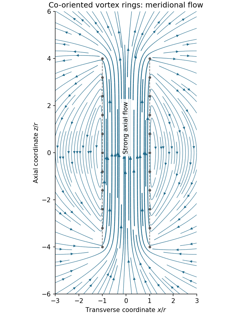
Assume all rings have the same circulation and orientation, and that there is no imposed background flow. Vortex lines describe the direction of vorticity, not the direction of velocity. For an incompressible fluid, the velocity induced by a thin vortex filament has the same Biot-Savart integral form as the magnetic field of a current filament:A closely spaced coaxial array of vortex rings is therefore analogous to a solenoid. The velocity field passes along the common axis through the rings and returns outside a finite array. Its orientation reverses if every circulation is reversed. In a long array, far from its ends and vortex cores, the velocity field of a dense coaxial vortex-ring array is approximatelyThe exterior field is exactly zero only in the ideal continuous infinitely long limit, with the background velocity set to zero. In a finite array the streamlines spread out at one end, run back outside, and converge into the other. A large number of closely spaced rings alone does not guarantee that the total array length greatly exceeds ; if it does not, the end and return flows remain substantial. Different unspecified ring circulations would require superposing their actual signed contributions.

Past exam of the physics B course of the University of Cambridge 2017 Paper 2 Section A A4 Solution 2026-10-18
The symmetry is electromagnetic reciprocity applied to mutual inductance. For thin closed circuits in vacuum, the magnetic vector potential generated by circuit B isStokes theorem converts the magnetic flux through circuit A into its magnetic vector potential circulation. Dividing by gives Neumann's mutual-inductance formula,The dot product and separation are unchanged by interchanging A and B, soEach has units . The winding orientations must be used consistently to determine the common sign. The same reciprocity holds in ordinary linear reciprocal magnetic media; it is not an unrestricted statement about biased nonreciprocal materials. Equivalently, a reversible magnetic energy function has equal mixed derivatives with respect to the two currents.
There are unlisted articles, also show them or only show them.