
Past exam of the physics B course of the University of Cambridge 2018 Paper 1 Section B B7 Solution 2026-10-18
The field law. In the Biot-Savart law, is the contribution to the magnetic flux density at the observation point from a directed wire element carrying steady conventional electric current . The vector points from that element to the observation point, , and . The constant is the vacuum permeability; the cross product sets the direction by the right-hand rule. Integrating the elements gives the total field, in teslas.
Past exam of the physics B course of the University of Cambridge 2018 Paper 1 Section B B6 Solution 2026-10-18
The boundary-value method. In a charge-free region, the electric potential obeys the Laplace equation, , and . Conductors impose equipotential boundaries, with specified voltages or charges, and a far-field condition fixes the remaining behaviour. The Uniqueness of the Dirichlet problem guarantees that a solution meeting the prescribed conductor potentials is the physical one. To see why, the difference of two candidate solutions is harmonic and vanishes on the boundaries; integration by parts gives , hence no difference in their fields. An exterior problem also needs the appropriate condition at infinity.
Two axisymmetric harmonic functions. For in spherical coordinates, the Laplacian reduces toFor , the bracket is . For , it is . ThereforeThe second function is singular at the origin, which is allowed here because that point lies inside the excluded conductor. The printed spherical Laplacian has a typo in its azimuthal term: its denominator should be . Both functions are axisymmetric, so that term vanishes and the typo does not affect these calculations.
Potential and field geometry. Set the lower conductor to zero potential and the distant upper plate to . The small boss sees approximately uniform background field , where . Combining the two harmonic functions to make on gives the conducting hemispherical protrusion in a uniform field,It also vanishes on the surrounding plane . The electric field components areEquipotentials crowd near the apex, and field lines meet the conductor normally.
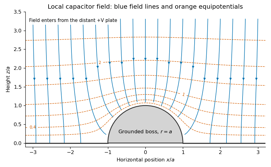
Original calculated local equipotentials and electric-field lines above the hemispherical boss; this is the small-boss approximation rather than an exact finite-gap solution
. Details. 
The formula has the correct uniform far field but does not exactly impose a flat upper equipotential at finite . It is the leading approximation justified by ; an exact finite-gap solution would include further corrections.
Past exam of the physics B course of the University of Cambridge 2018 Paper 1 Section A A5 Solution 2026-10-18
Apply equal compressive pressure in all directions; here denotes Poisson's ratio. The three principal normal stresses are . For an isotropic linearly elastic material, Hooke's law givesand similarly for . At small strain, the fractional volume change is the sum of these normal strains:The bulk modulus is , giving the isotropic elastic modulus relation,The result assumes linear elasticity and fixed isotropic moduli. In the incompressible limit with finite Young's modulus, the bulk modulus tends to infinity.
Past exam of the physics B course of the University of Cambridge 2018 Paper 1 Section A A4 Solution 2026-10-18
The conventional electron plasma frequency isUse , , and . ThenThe equal proton density ensures charge neutrality; it does not double the electron density in this formula. Protons have their own plasma frequency,If both cold species are allowed to move in the relative charge-separation oscillation, its squared frequency is . This gives , only about above the electron-only answer, because .
Past exam of the physics B course of the University of Cambridge 2018 Paper 1 Section A A3 Solution 2026-10-18
A large gas volume can reduce the effective mass density of the water surrounding the hull. In the simple quasihydrostatic model for the buoyancy of an aerated liquid, gas void fraction givesBy Archimedes' principle, a boat displacing volume then has buoyant force . To support the same boat mass , it needs a larger displaced volume , so its draft increases. If that exceeds the available watertight displacement, it can lose flotation or become swamped:Uneven aeration and strong plume motion can also disturb stability. This explains a possible hazard, not a claim that any bubble plume must sink a boat: upward water flow, turbulence and the distribution of bubbles can exert substantial additional forces.
Past exam of the physics B course of the University of Cambridge 2018 Paper 1 Section A A2 Solution 2026-10-18
Let the signed axial velocity on the axis be . Smooth axisymmetric flow has and regular radial velocity at . The incompressible flow condition in cylindrical coordinates isTo leading order near the axis, integrate from zero to . The integration constant vanishes by regularity, giving the near-axis radial velocity in incompressible axisymmetric flow,With the usual signed interpretation ,For this is outward: the outward axial flow slows as its distance from the origin grows, and incompressibility requires radial spreading. Here has units , so the answer is a speed.
Past exam of the physics B course of the University of Cambridge 2018 Paper 1 Section A A1 Solution 2026-10-18
An infinite sheet of surface charge density gives an electric field of magnitude on either side, normal to the sheet and directed away from positive charge. Use the superposition principle for the two sheets. Choose normals for and for . Away from the charged planes,The minus sign on the second contribution makes its field point toward the negatively charged sheet. Each sector has a uniform electric field; its direction changes on crossing a sheet.
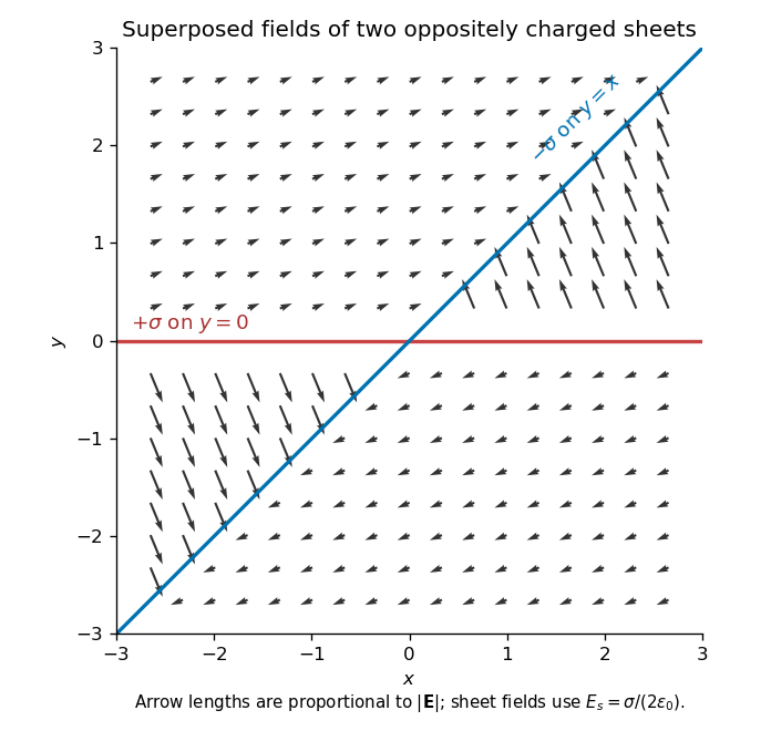
Original calculated electric-field directions for the intersecting positive and negative charge sheets; arrows retain the relative field magnitudes in the four sectors
. Details. 
For example, above both sheets the field points right and slightly upward, whereas in the sector but it points left and steeply upward. The other two sectors follow by inversion through the origin. The normal field jumps by the appropriate surface charge divided by ; a single field value on an ideal zero-thickness charged sheet is not required.
Past exam of the physics B course of the University of Cambridge 2017 Paper 2 Section C C13 Solution 2026-10-18
Molecular transport across gradients. A gas can transport momentum, thermal energy and species abundance even when its average bulk velocity is zero. Molecules arriving at a point carry properties acquired near their preceding collisions. A small gradient makes the populations arriving from opposite sides slightly different, producing transport from larger to smaller values of the carried property. A continuum transport law requires a mean free path small compared with the gradient length, and relaxation times short compared with the observation time.
For a dilute hard-sphere gas,where is molecular collision diameter. Both speed and collision distance matter: high speed alone does not determine a transport coefficient.
A simple kinetic estimate makes the common structure explicit. For a quantity carried per particle, a molecule moving at angle to brings approximately . Expanding to first order and averaging an isotropic velocity distribution givessince and . This mean-free-path argument estimates the coefficients; a detailed collision calculation changes their numerical prefactors and distinguishes different relaxation rates.
Momentum transport and viscosity. For a shear flow with mean velocity , the transported directed momentum per molecule is . The net flux of momentum in the direction isHere is dynamic viscosity in . The associated shear stress on a material surface has the corresponding traction sign convention; the flux carries momentum from the faster-moving layer towards the slower-moving one. The kinematic viscosity is , with units . Viscosity smooths velocity gradients, and the lost ordered mechanical energy becomes heat.
Heat transport. Let be the thermal heat capacity per molecule, in . Substituting gives Fourier's law,Thermal conductivity has units . For a monatomic gas, translational equipartition gives . Rotational or vibrational excitations in other gases can increase the energy carried per molecule, while collisions govern how those modes exchange energy. A temperature gradient can therefore be transported differently from directed momentum even when the dimensional estimates look similar.
Species transport. For a dilute tracer or a mixture with prescribed total density and negligible bulk flow, molecules diffuse down concentration gradients. The first-gradient number flux is Fick's first law,The diffusivity has units ; multiplying number flux by the species mass gives mass flux. More generally one uses diffusion flux relative to the mixture's bulk velocity and specifies mass or mole fractions. The approximation is not a claim that an arbitrary pure-gas pressure gradient can remain at rest while only a Fick flux acts. In a mixture, collision cross-sections and relative molecular speeds, including the reduced mass, determine the species diffusivities.
Dependence on density and temperature. The kinetic estimates of gas transport coefficients predict, for fixed collision diameter and molecular heat capacity,Thus dynamic viscosity and thermal conductivity are approximately density independent in the dilute continuum regime. Reducing density reduces the number of carriers but increases their mean free path in the same proportion. At fixed density all three estimates grow as ; at fixed pressure, andKinematic viscosity and thermal diffusivity also grow roughly as at fixed pressure in this model. Real interaction potentials make effective collision cross-sections temperature dependent, and internal excitations change . Dense-gas correlations and boundaries invalidate the simple cancellation. In particular, when the mean free path approaches the apparatus scale, transport becomes free molecular; it cannot be described by extending the same local, pressure-independent Fourier and viscosity coefficients indefinitely.
Heat diffusion equation. For a stationary gas with constant volumetric heat capacity , constant thermal conductivity and negligible compression work, the energy balance in any fixed volume isHere is a possible heat generation rate per volume. The divergence theorem and Fourier's law yieldThermal diffusivity has units and is of order . In a moving or compressing gas, the material derivative, pressure-volume work and viscous heating must also enter the internal-energy equation. The displayed pure diffusion equation describes the approximation in which those effects are absent or negligible.
Representative solutions. With no source, a steady one-dimensional slab between temperatures at has and uniform heat flux . Thus a constant spatial gradient transports heat without changing local temperature in time when the boundaries continually supply and remove it.
For an infinite medium and an initial sinusoidal temperature perturbation,Short spatial wavelengths decay faster, and the characteristic smoothing length after time is . A finite slab with both ends held at has a sine expansion with factors ; its slowest relaxation time is .
An instantaneous heat input per unit transverse area at in an otherwise uniform infinite medium gives the Gaussian solutionIts integral conserves the deposited heat. The peak falls as while its width grows as ; diffusion redistributes energy instead of transporting a sharp front at a single velocity.
Finally, a semi-infinite body initially at and held at surface temperature from hasIt has and approaches far from the boundary at finite time. These solutions demonstrate steady conduction, mode decay, spreading of localized heat and boundary-driven diffusion. Their idealized behaviour at extremely short times or arbitrarily long distances must be interpreted within the continuum regime rather than as an assertion of instantaneous microscopic communication.
Past exam of the physics B course of the University of Cambridge 2017 Paper 2 Section C C12 Solution 2026-10-18
For a classical dilute ideal gas in thermal equilibrium, the probability of a single-particle velocity is proportional to the Boltzmann factor for kinetic energy, . Velocities with speed between and fill a spherical shell of velocity-space volume . The normalized Maxwell speed distribution is thereforeThe factor counts states, rather than representing an extra Boltzmann energy factor.
Set and use . Normalization cancels in ratios, so the given recurrence givesConsequentlyThe root mean square speed is larger than the mean speed, consistent with the positive variance of the speed distribution.
There are unlisted articles, also show them or only show them.