
Shielded toroidal-flux electron interference Created 2026-10-18 Updated 2026-10-20
In 1986, Akira Tonomura and collaborators coated a ferromagnet shaped as a torus with superconducting niobium and copper. A cooled stage held it in a 150 kV field-emission electron microscope. An electron biprism overlapped object and reference waves; film holograms were reconstructed optically. Room-temperature leakage screening selected samples; varying copper thickness tested electron penetration.[ref]
Below the superconducting transition, through-hole and outside electron waves differed in wave phase by zero or modulo . Warming through it changed the interference reversibly. Leakage and coherent-penetration bounds do not prove zero magnetic field.[ref]
Evidence for Aharonov-Bohm effect with magnetic field completely shielded from electron wave by Akira Tonomura and others. p. 794, Figs. 6–7: experimental limits
Why these two phases? The shield's superconducting flux quantum is , whereas the probing electron has electric charge . Substituting givesAn odd therefore moves a carrier fringe by half its spacing; an even leaves it unchanged modulo a full spacing. The phase quantization provides an internal check on the superconducting enclosure. It does not mean that zero wave phase proves zero trapped magnetic flux.[ref]
The Aharonov-Bohm effect and its applications to electron phase microscopy by Akira Tonomura. 2006, p. 49, Confirmation experiments on the AB effect; Fig. 2 on p. 48
The readout is electron holography in the off-axis holography geometry: a known tilted reference converts an unknown relative wave phase into a spatial carrier displacement. Reconstructing a magnetic wave phase assumes stable reference phase, adequate coherence and a calibrated carrier; electrostatic charging and material traversal can also shift wave phase. Optical wave phase amplification rescales the displayed fringe displacement. The experiment's shielding and comparison tests support the magnetic inference; an interferogram by itself measures the total relative wave phase, rather than separately certifying every contribution. The ideal field-free model describes the limiting geometry, while finite leakage and penetration remain questions of experimental bounds.
Magnetic flux spectrum of a quantum ring Created 2026-10-18 Updated 2026-11-05
For circumference and Hamiltonian operator with a periodic boundary condition, the plane waves have energies , where and . Minimal coupling gives , where is the magnetic flux oriented consistently with increasing position around the ring. The ordered spectrum is periodic in with period one, corresponding to magnetic flux quantum .
On , its lowest two energies are and . Their crossings at half-integer can be opened by a potential that couples the relevant momentum states.
Folium of Descartes 2026-10-18
For nonzero real , the folium of Descartes is the algebraic curve , with rational parametrization of an algebraic curveIt is symmetric about and has a node at the origin, with the coordinate axes as tangents. For , traces a loop in the first quadrant, returning to the origin as . Its enclosed area, by Green's theorem, isThe other branches approach the asymptote as . Negative rotates the positive- picture through .
Abrikosov vortex lattice 2026-10-18
A periodic array of Abrikosov vortices. In the isotropic local theory near the upper critical magnetic field, the triangular array has a lower Helmholtz free energy than the square array.[ref]
Nobel Lecture: Type-II superconductors and the vortex lattice by Alexei Alexeyevich Abrikosov. p.976, equations3–4 and the two lattice geometries
The useful distinction is between vortex existence, array geometry, and vortex mobility. Quantized winding does not force every array to be triangular or defect-free. A stationary array and vortices moving under an applied electric current also have different transport consequences; flux pinning matters for carrying useful electric currents.
Tensile modulus experiment Created 2026-10-18 Updated 2026-10-20
MIT's Spring 2004 laboratory assignment Properties of Heat Treated Steel gives a concrete tensile testing protocol. Record transducer channels and calibration factors; measure specimen diameter and length, and the extensometer gauge length with its locking pin inserted. Zero the load cell, pin the threaded grips into their adapters, and attach the extensometer centrally. Apply the specified seating load, record actuator position, then acquire readings every second while moving at about . The handout derives engineering stress from load cell force, engineering strain from extensometer deformation, and Young's modulus by linear regression below the proportional limit; it warns that actuator-derived strain includes apparatus deformation.[ref]
Properties of Heat Treated Steel by Massachusetts Institute of Technology. Laboratory assignment 10, printed pp. 2–3: Procedure for Tension Tests; Calculations
For a modulus-focused measurement, select a load window after seating, hold temperature and loading rate consistent, and record force, local extension and crosshead displacement together. Fit within that window and calculate . Inspect the regression residuals for curvature; repeat at a lower maximum load and include unloading to check elastic deformation. These are diagnostic additions to the cited protocol, whose full test continues through failure. The handout's seating load is specific to its specimens and apparatus, rather than a universal preload.
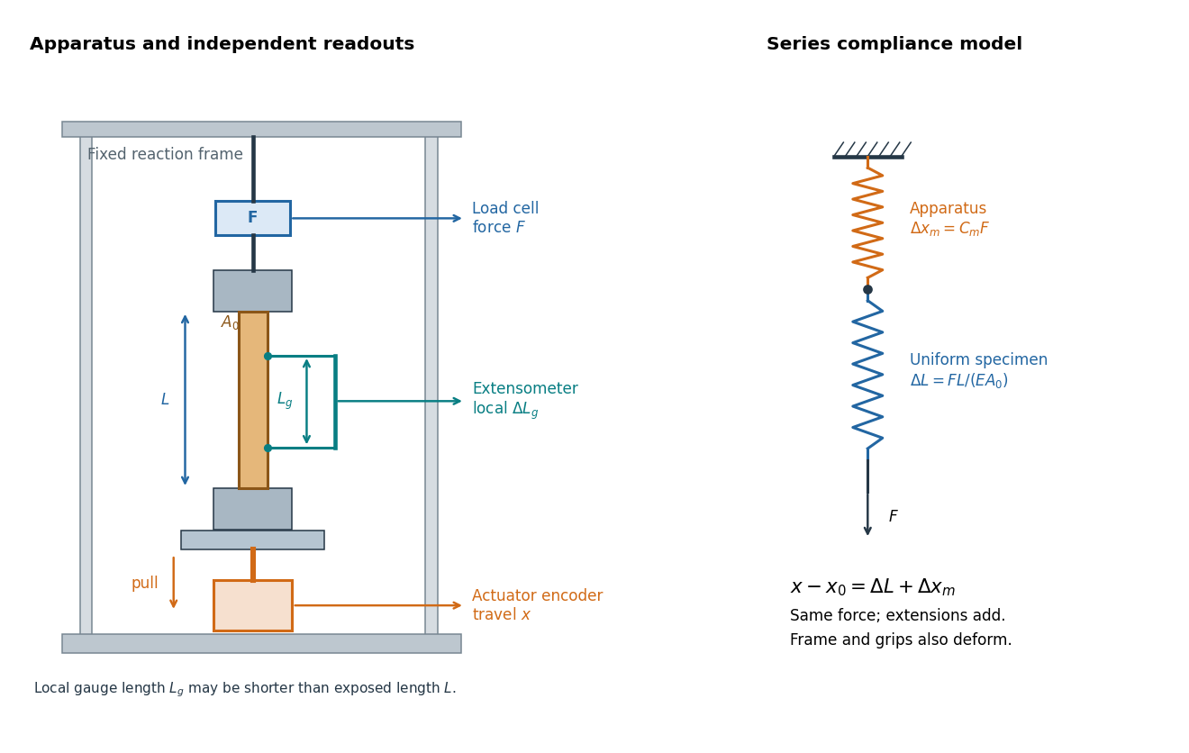

An extensometer measures the change between its contact points; crosshead displacement measures travel of the machine's moving member. The manufacturer Instron explicitly distinguishes local strain from travel that includes machine deformation and machine compliance.[ref]
Static Axial Clip-On Extensometers by Instron. FAQs: How does a clip-on extensometer work?; When should I use a clip-on extensometer instead of crosshead displacement?
The gauge length can be shorter than the uniform length between grips. Thus even a perfectly rigid machine generally has : the local instrument sees only its own segment. Do not divide one channel's extension by the other channel's reference length.Grips must transmit axial force without slip. Misalignment adds bending moment and makes opposite sides experience different axial strains; an instrument on just one side may then report a biased modulus. A changing extension offset, hysteresis between loading and unloading, or load-dependent fitted slope is evidence to investigate seating, slip or material response. A straight line over a short interval alone does not identify which is responsible.
Work by Yen-Chi Chen 2026-10-18
Physics course of the year 4 of the natural sciences course of the University of Cambridge Created 2026-10-18 Updated 2026-10-20
Physics course of the year 3 of the natural sciences course of the University of Cambridge Created 2026-10-18 Updated 2026-10-20
Physics course of the year 2 of the natural sciences course of the University of Cambridge Created 2026-10-18 Updated 2026-10-20
Physics course of the year 1 of the natural sciences course of the University of Cambridge Created 2026-10-18 Updated 2026-10-20
Gauge boson self-interaction Created 2026-10-18 Updated 2026-10-20
Gauge boson self-interactions arise from the quadratic-field term in a non-Abelian gauge field strength. Squaring that field strength in the Lagrangian yields cubic and quartic pure-gauge interaction vertices. Higher-point scattering can occur by connecting these vertices, even without a corresponding fundamental higher-valence vertex.
Characteristic X-ray Created 2026-10-18 Updated 2026-10-20
A Characteristic X-ray comes from an electronic transition filling an inner electron shell vacancy. The emitted photon carries the difference between atomic energies. Vacancy creation by direct electron impact requires kinetic energy above the shell's binding energy, exceeding the line energy. Higher tube voltage need not move the spectral line.[ref]
Chapter 5: X-Ray Production (teaching slides) by K. P. Maher. Diagnostic Radiology Physics: A Handbook for Teachers and Students; IAEA Chapter 5, §§5.2.2–5.2.3: shell vacancy, binding-energy threshold and characteristic radiation
An original stipulated shell model illustrates the distinction without using measured atomic data. Let positive binding energies be and , ignoring relaxation corrections. Filling a K-shell vacancy from the L shell releasesAn tube can energetically emit a bremsstrahlung photon, yet cannot directly remove this K-shell electron. A tube can create that vacancy by electron impact; if radiative filling occurs, the line is still , not . This argument concerns direct electron impact and an initially unexcited target; it does not describe every possible excitation route.
X-ray tube cutoff Created 2026-10-18 Updated 2026-10-20
For an electron starting with negligible kinetic energy and accelerated through a constant positive electric potential difference , electrical work supplies . In the ideal single-electron bremsstrahlung model, conservation of energy bounds any one emitted photon:The endpoint corresponds to essentially all available kinetic energy going into one photon. It is a limiting bound, not a claim that every electron produces an endpoint photon. Neglect target recoil, initial kinetic energy, and losses before the emitting interaction. If the accelerating voltage varies, its largest value sets the corresponding ideal upper endpoint; a mean voltage does not substitute for that value.
For a calculated constant- example, gives and . Doubling halves . Producing a photon requires at least in this model. A continuous frequency spectrum spans lower photon energies; the cutoff calculation predicts neither its shape nor the efficiency of photon emission.
On-off X-ray photon counting 2026-10-18
Background subtraction must account for uncertainty in the background measurement itself. In an original idealized experiment, an on-source exposure contains source and background, while an independent off-source exposure contains background alone. Assume stationary rates and identical background acceptance per unit live time. With , let independent counts obey Poisson distributions:Then linearity of expectation and addition of variances for independent random variables giveThe result concerns accepted source counts , after all efficiencies. For large counts the normal approximation gives the descriptive signal-to-noise ratio in photon countingThis plug-in ratio is not an exact null-hypothesis significance. Small counts require the discrete Poisson model; searching many sky directions also changes a detection claim's p-value.
Choose and , with observed counts and . Thus , , and the estimated standard deviation is counts. The inferred uses the preceding and includes counting uncertainty only. The descriptive ratio is . Treating the scaled off-source background as exact would omit 200 counts squared from the estimated variance.
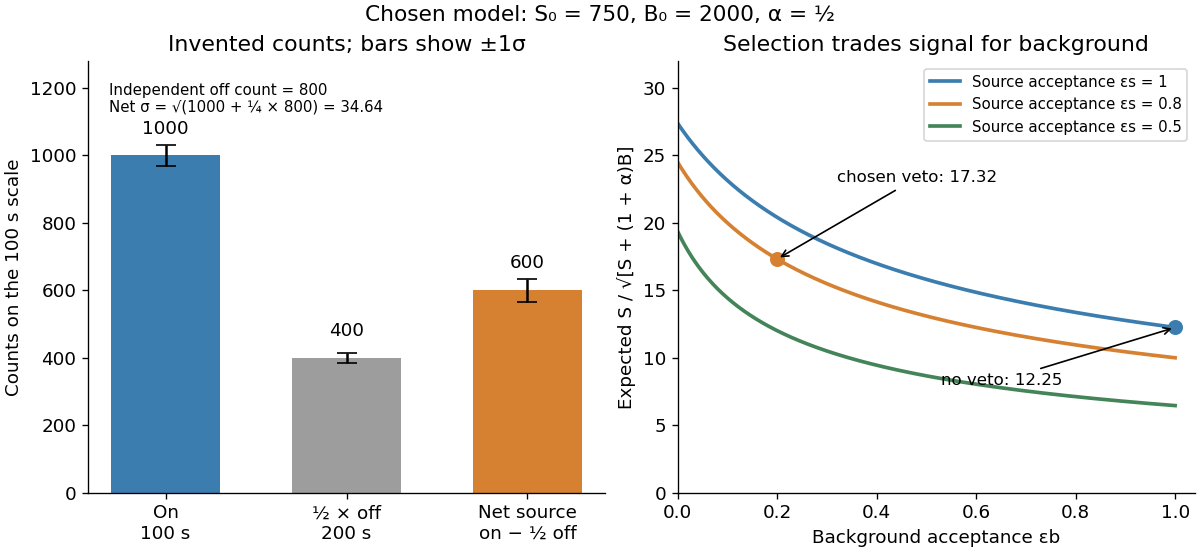
Invented on-off counts and the effect of background rejection
. All numbers are chosen teaching values, not historical measurements. Independent off-source counts contribute uncertainty. The rejection curves hold the source acceptance fixed within each labelled case. Details.
For a selection-design comparison, suppose before a veto the expected source contribution is , the on-source background is , and . Let source acceptance be and background acceptance be . Then , , and , whereas omitting the veto gives . Rejection helps because the background is reduced enough to compensate for lost source events. A different veto can make matters worse; source efficiency and background rejection are separate probabilities. This comparison is an independent teaching example, not the efficiency calibration used above.
Absorption edge 2026-10-18
An absorption edge is an abrupt change in photon absorption as incident photon energy crosses an electronic excitation threshold. For inner-shell photoionization, a new vacancy-production channel opens near the shell's binding energy. This threshold concerns incident energy; a Characteristic X-ray concerns a subsequent difference of atomic energies. They are different observations. Barkla's lecture explicitly treats characteristic emission as requiring a critical excitation condition, while discussing characteristic radiation separately from scattering.[ref]
Characteristic Röntgen Radiation by Charles Glover Barkla. Nobel Lectures, Physics 1901–1921; Barkla, Characteristic Röntgen radiation, printed p. 395, PDF p. 135: shorter-wavelength excitation and critical condition
In the stipulated X-ray fluorescence model, the K threshold is , whereas the K lines are and . An absorber made of a different material could have its own absorption edge between those line energies, preferentially removing the upper line. Actual near-edge structure and attenuation values require material data; the following deliberately chosen coefficients are not such data.
Beam hardening 2026-10-18
An original two-energy model demonstrates the failure of a single constant linear attenuation coefficient for a mixed beam. Suppose the two components contribute equally to the empty-path detector signal and have stipulated and . With fixed linear detector response and no accepted scattering of light,The initial slope corresponds to , but at , , rather than . The more strongly attenuated component disappears faster. If that component has lower photon energy, the surviving beam has a higher mean energy: beam hardening. The formula is explicitly a two-component example, not a universal rule that attenuation decreases monotonically with photon energy. Detector weighting also matters when interpreting a broadband transmission signal.
Half-value layer 2026-10-18
The half-value layer is the thickness reducing the specified transmitted signal by one half. For constant monoenergetic linear attenuation coefficient , solving gives . The stipulated gives ; two such layers transmit one quarter. A broad frequency spectrum need not retain the same half-value layer after filtering.
Linear attenuation coefficient 2026-10-18
The linear attenuation coefficient is the infinitesimal probability of removal from the uncollided beam per unit path length. Its units are inverse length. In the homogeneous monoenergetic model, ; is the thickness leaving fraction uncollided. The mass attenuation coefficient is for material mass density . Removing a photon by scattering of light does not imply deposition of all its energy at that point; attenuation and energy absorption are different quantities.[ref]
2. The Mass Attenuation Coefficient. Tables of X-Ray Mass Attenuation Coefficients and Mass Energy-Absorption Coefficients by John H. Hubbell and Stephen M. Seltzer; NIST §2, mass thickness, Eq. (1), and total interaction cross section; distinction from the mass energy-absorption coefficient
There are unlisted articles, also show them or only show them.