
Skew-Hermitian decomposition of a unitary matrix Created 2026-10-18 Updated 2026-11-05
The displayed parts of a unitary matrix are skew-Hermitian matrices. Expanding gives and . They admit a common orthonormal eigenbasis. For a unitary eigenvalue , the corresponding part eigenvalues are and . If , then , so these are exactly its real and imaginary parts and both are real skew-symmetric matrices. Such an invertible antisymmetric matrix has even dimension, by its determinant. If one part has distinct eigenvalues, commutation alone shows its one-dimensional eigenspaces are preserved by the other part.
Power broadening 2026-10-18
In the two-level saturation population model, and the population-difference reduction reach half their resonant values at . Their half width at half maximum is therefore and their full width at half maximum is in angular frequency, or in hertz. This is power broadening: stronger excitation addresses a wider range of detunings even though the lifetime has not changed.
Increasing improves the local population-difference reduction but broadens the response. From to , this reduction increases from to , while the width increases from to . The contrast approaches a limit and the width keeps growing. This single-atom width is not automatically the width of a velocity-averaged pump–probe feature.
For example, if the distribution of velocities is approximately constant across the narrow resonant classes, the population-only overlap integral contains two Lorentzian line shapes: a probe of half width and a pump hole of half width . Their centres in are separated by . The convolution of these profiles has half width in that separation, so its full width at half maximum as a function of is . Even this simplified pump–probe width differs from the single-atom power broadening formula. Finite Doppler broadening and coherent or multilevel effects require further analysis.
For in a two-dimensional infinite square well, the lowest two states are and , both nondegenerate. The next energy is the smaller of and : every other candidate lies above at least one of these. Requiring equality gives , or . In units the lowest distinct energies are then , and , with degeneracies one, one and two. The third-level pair is exactly and .
Patrick Maynard Stuart Blackett and Giuseppe Occhialini began their cosmic-ray collaboration in 1931. They used the coincidence methods of Walther Bothe and Bruno Rossi to make a particle initiate its own recording. Blackett later reported tracks on about of their counter-controlled photographs, compared with roughly – for random expansions in small chambers. Those figures describe the reported apparatus and conditions, not a universal detection efficiency.[ref]
Cloud Chamber Researches in Nuclear Physics and Cosmic Radiation by Patrick Maynard Stuart Blackett. Cloud chamber researches in nuclear physics and cosmic radiation, lecture 13 December 1948, pp. 104–105: collaboration, coincidence precedent and photographic yield
In their 1933 account, Geiger counters above and below the chamber fed a coincidence circuit. Its pulse operated a thyratron, magnet and spring-release valve, letting a light piston expand the gas. A mercury-vapor lamp then illuminated the drops. A water-cooled solenoid supplied the magnetic field; two oblique cameras allowed track reconstruction. Moving the lower counter changed which trajectories could be recorded.[ref]
Some Photographs of the Tracks of Penetrating Radiation by Patrick Maynard Stuart Blackett and Giuseppe Paolo Stanislao Occhialini. Some Photographs of the Tracks of Penetrating Radiation, pp. 699–701, section 1 and Fig. 2; p. 719, Description of Plates: expansion sequence, cameras and alternate counter position
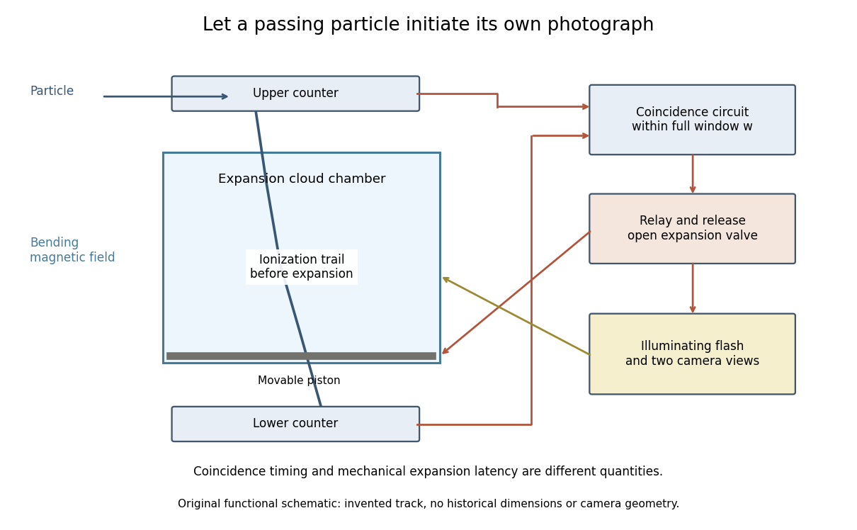
Counter coincidence initiates expansion, illumination and photography in a functional reconstruction of the Blackett-Occhialini method
. Original diagram, not a scale drawing or a historical photograph. The pictured track and positions are illustrative; magnetic curvature and event direction require further measurements. Details.Two timing problems must be separated. The coincidence circuit's window distinguishes nearly simultaneous counter signals. The mechanical expansion latency determines how much the existing ionization trail spreads before droplets form. For a chosen one-coordinate diffusion model with initial variance , diffusion coefficient and expansion delay ,Taking , and gives . This is an original illustrative calculation, not the historical track width. It shows why a fast electronic pulse does not by itself guarantee a sharp photograph: the subsequent mechanical response also matters.
The photographs revealed groups containing positive and negative electron-like tracks, complementing the Anderson positron track experiment. Their interpretation depended on track curvature, direction, ionization and particle range, not simply on the presence of a coincidence.[ref]
Some Photographs of the Tracks of Penetrating Radiation by Patrick Maynard Stuart Blackett and Giuseppe Paolo Stanislao Occhialini. Some Photographs of the Tracks of Penetrating Radiation, pp. 702–708 and p. 718, Summary: associated tracks and evidence for positive electrons
Blackett explicitly noted that the counter control favored larger particle showers.[ref]Cloud Chamber Researches in Nuclear Physics and Cosmic Radiation by Patrick Maynard Stuart Blackett. Cloud chamber researches in nuclear physics and cosmic radiation, p. 108: multiplicity-dependent triggering and overrepresentation of large showers
The multiplicity bias from a detector trigger gives a small model of that effect: a recording method can improve the study of rare interactions while making its photographs unrepresentative of the incident population. Triangular solve 2026-10-18
A triangular solve computes the unique solution of a linear system for an invertible triangular system using forward substitution for a lower triangular matrix or backward substitution in a triangular system for an upper triangular matrix.
Motional sideband 2026-10-18
A motional sideband is a transition that changes internal excitation and a motional quantum number together. Define the internal energy gap as . A carrier drives ; the first red sideband drives ; the first blue sideband drives . Their resonant drive angular frequencies follow by subtracting these energy levels. For a Raman transition, the drive is a beam-difference frequency with a sign fixed by the selected internal transition.
Choose a real carrier Rabi angular frequency defined so that resonant carrier excitation is . In the Lamb-Dicke regime, isolated first-sideband Hamiltonians in a rotating frame can be written, after choosing the pulse phase, asThese formulas use a rotating-wave approximation: neglected carrier and other-sideband terms oscillate rapidly compared with the retained coupling. The drive's effective width and sideband coupling must be small compared with ; sufficient suppression of off-resonant carrier excitation must also be checked. The red interaction is a Jaynes-Cummings model with a motional quantum replacing a cavity photon. The blue interaction creates internal excitation and a motional quantum together; the external laser supplies energy. The driven-system rotating-frame Hamiltonian alone is not the total laboratory energy.
Lamb-Dicke regime Created 2026-10-18 Updated 2026-10-20
The Lamb-Dicke regime means the wave-induced phase change across the occupied motional wavepacket is small. For one normal mode, let be the ground state's position standard deviation, and write using creation and annihilation operators. Here is mass and the Planck constant divided by . The effective wave vector component is the single beam's component for a direct transition, or the difference of two beam components for a Raman transition. With dimensionless , the useful condition is over the populated number states, rather than merely .
Absorb the sign of into the pulse phase. Expanding the coupling factor givesThe constant term preserves ; the annihilation operator gives ; the creation operator gives . The different square roots explain why removing a motional quantum becomes impossible at , while adding one remains possible. Smallness of controls this spatial expansion; resolving the resulting transitions is a separate frequency requirement.
Consider an original electrical circuit model between two equipotential cross-sections. A normal path has electrical resistance . Let indicate whether an additional path connects those same cross-sections; when connected it has electrical resistance . Ideal voltage contacts measure those cross-sections. This collapses a spatial network to two parallel branches; it is not a fit to the Bednorz-Müller experiment.
For , both branches have the same electric potential difference . Ohm's law and the Kirchhoff node law give , henceThe last case follows directly from the ideal short's constraint , provided it can carry the imposed electric current below its superconducting critical current. It does not follow by substituting into . A normal bridge in series with otherwise superconducting pieces belongs in ; superconducting grains alone need not short the measured interval.
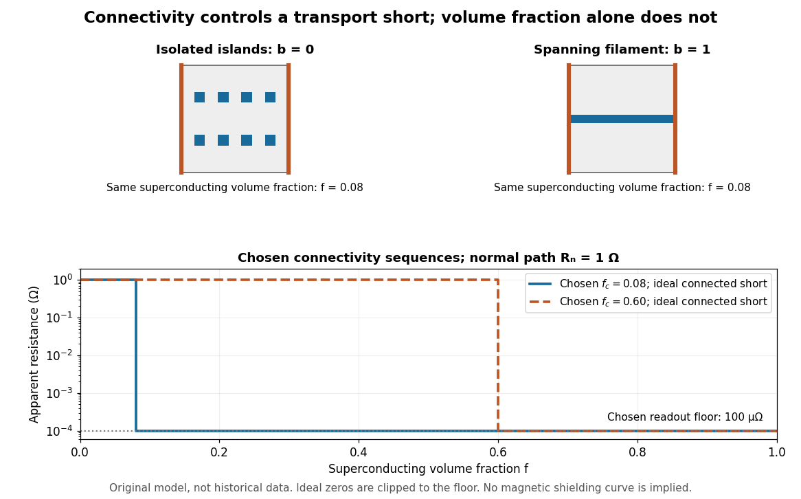
Equal superconducting volume fractions can have different transport connectivity
. Original chosen geometry and circuit example, not measured data or a historical fit. Top: blue superconducting regions between orange equipotential ends, taken uniform through the thickness, have superconducting phase fraction . Bottom: two stipulated connectivity thresholds, and , produce different apparent electrical resistance drops. Ideal zero values are displayed at a chosen instrument floor; these curves predict neither magnetic susceptibility nor a universal percolation threshold. Details.Choose . A connected bridge with gives , almost a hundredfold drop despite finite electrical resistance. An ideal connected superconducting filament instead gives zero in this model even when its volume is a small part of the specimen. Isolated superconducting islands can have the same superconducting phase fraction while leaving . For the illustrative disconnected geometry we stipulate that the normal conducting network retains .
To plot a chosen connectivity sequence, set for and for , with on the connected branch. The two displayed values of describe different chosen architectures. A real percolation calculation would need an explicit network and spatial distribution; the scalar phase fraction does not determine by itself.
An instrument with unresolved electric potential difference bounded by reports only . For chosen and this floor is , assuming offsets and noise are included in the bound. The figure clips smaller model values to that floor. Increasing improves this formal bound only while Joule heating and the path's superconducting critical current remain controlled. None of these transport statements determines the superconducting phase fraction or establishes complete Meissner effect shielding.
Tail-anchored protein 2026-10-18
A tail-anchored protein has a membrane-spanning segment near its C-terminus; many reach the endoplasmic reticulum after biological translation.
Sec61 complex 2026-10-18
The Sec61 complex supports passage across the endoplasmic reticulum membrane and lateral entry of membrane-spanning segments into its lipid bilayer.[ref]
Membrane Protein Insertion at the Endoplasmic Reticulum by Sichen Shao and Ramanujan S. Hegde. Shao and Hegde, 2011; “The Sec61 Translocon”, Figure 4
History of total variation of a function 2026-10-18
Camille Jordan developed bounded variation as part of his work in real analysis; his treatment of functions and arc length was part of the influence of his analysis textbooks.[ref]
Marie Ennemond Camille Jordan by John Joseph O'Connor and Edmund Frederick Robertson. Discussion of Jordan's analysis textbooks, bounded variation and definition of curve length; biography by J. J. O'Connor and E. F. Robertson, last updated March 2001
The Jordan decomposition of a function of bounded variation expresses the underlying idea especially well: complicated changes of direction can be separated into two functions that only increase.Let have bounded variation, and let be continuous functions on . In any tagged sum for the Riemann-Stieltjes integral,Taking the limit proves the displayed error bound. Thus approximating uniformly to accuracy controls this integration error by , even when the integrator is not differentiable. For the piecewise linear function in partition example of total variation, accuracy gives an error at most . Total variation supplies exactly the movement budget that an endpoint difference would miss.
For each positive integer , put on . Its supremum norm is exactly , so this sequence of functions converges to zero by uniform convergence. Nevertheless,Each of its complete sine oscillations contributes : rise from zero to , fall through zero to , then return to zero. Taking a partition of an interval through all extrema attains . Every further partition refinement merely subdivides monotone function segments, so the same reasoning as in partition example of total variation proves the upper bound too.
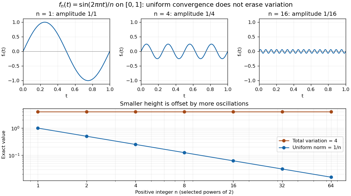
The functions sin(2πnt)/n converge uniformly to zero while their total variation remains 4; all three function plots use the same vertical scale
. Details. For a continuously differentiable function on a closed bounded interval, total variation also satisfiesApplied here, the derivative is , and integrating its absolute value over periods gives . The differentiability hypothesis matters: the partition definition applies much more widely than this derivative formula.[ref]
1 Algebraic and Analytic Methods. NIST Digital Library of Mathematical Functions; §1.4(v), equations 1.4.33–1.4.34, Functions of Bounded Variation
Small pointwise size and small accumulated movement are different approximation goals. Partition example of total variation Created 2026-10-18 Updated 2026-10-25
Define a piecewise linear function by joining the five points . Its net change is , but the increments at these knots are . Their absolute values giveThis is its exact total variation, not merely one lower bound. Given any partition of an interval, insert all five knots. The triangle inequality ensures that this partition refinement cannot decrease the sum. On each resulting monotone function segment, the absolute increments telescope, so every refined sum is . The knot partition of an interval itself attains .
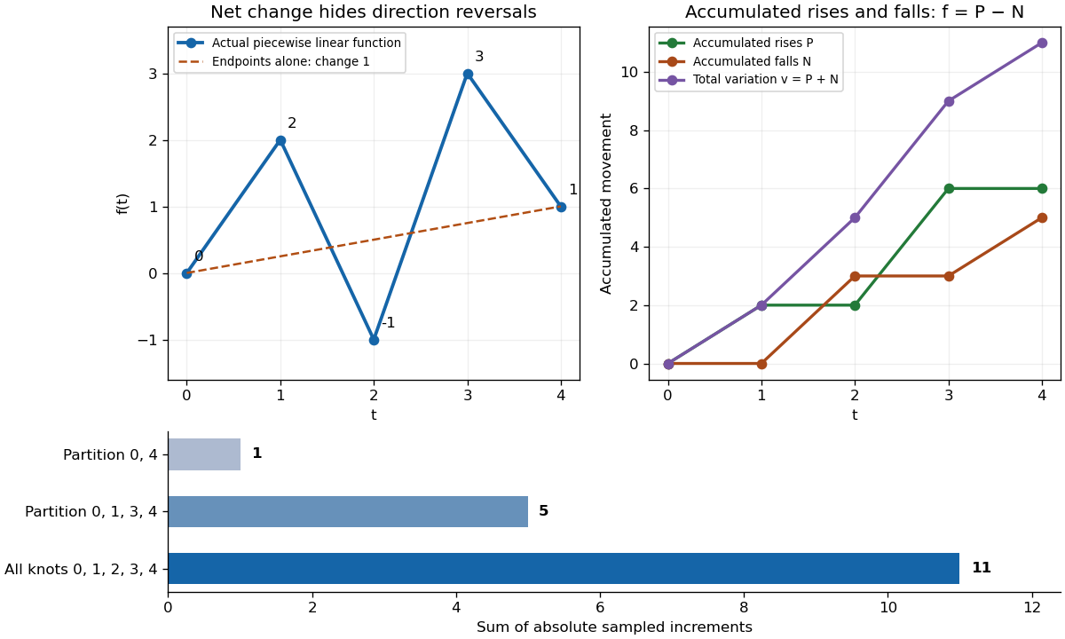


Sampling only at gives . Sampling at gives . Inserting the remaining knot at reveals the descent and rise that were hidden inside , giving . These are nested partitions of an interval: their sums increase because each is a partition refinement of the preceding one. Arbitrarily chosen unrelated partitions of an interval need not produce an increasing sequence of sums.
Angular impulse 2026-10-18
The time integral of torque about a specified origin equals the change in angular momentum about that origin under the usual fixed-origin inertial frame balance. Its units are , equivalently . For rotation about a fixed principal axis, the magnitude is .
Constant-power rotation against dry friction 2026-10-18
For positive angular velocity, a motor delivering constant mechanical power produces torque . With constant opposing kinetic friction torque , angular momentum balance gives the displayed equation and a steady speed . A small increase in speed reduces the driving torque below the friction torque, making this equilibrium stable within the model. The constant-power idealization is singular at exact rest and requires a separate starting regime in a real motor.
A rigid body's axial moment of inertia and a constant resisting torque give constant angular acceleration . Hence and the angular displacement is the displayed expression. Equivalently, the lost rotational kinetic energy equals the resisting work . The total number of revolutions is ; the number of whole revolutions completed is its floor function.
Corotating point-mass tidal field Created 2026-10-18 Updated 2026-10-20
Use local axes radial, tangential in the orbital plane, and perpendicular to that plane around a circular Kepler orbit with . The gravitational tidal tensor is . A uniformly corotating frame adds the gradient of centrifugal acceleration, , giving the displayed effective tensor for stationary offsets. Thus the radial differential acceleration is . These are accelerations, or forces per unit test mass; an actual differential force includes that mass. Moving offsets also experience Coriolis acceleration.
Stored excitation in a pulsed laser 2026-10-18
A short optical pulse can draw on previously stored excitation. In the original calculation below, , , , , and for , followed by . The cavity field initially remains small while pumping fills the upper state. Once sufficient gain develops, the photon population grows and depletes the stored inversion. Continuing pump action can refill it, giving relaxation oscillations in this simple model. This is not a fit to Maiman's recorded output.
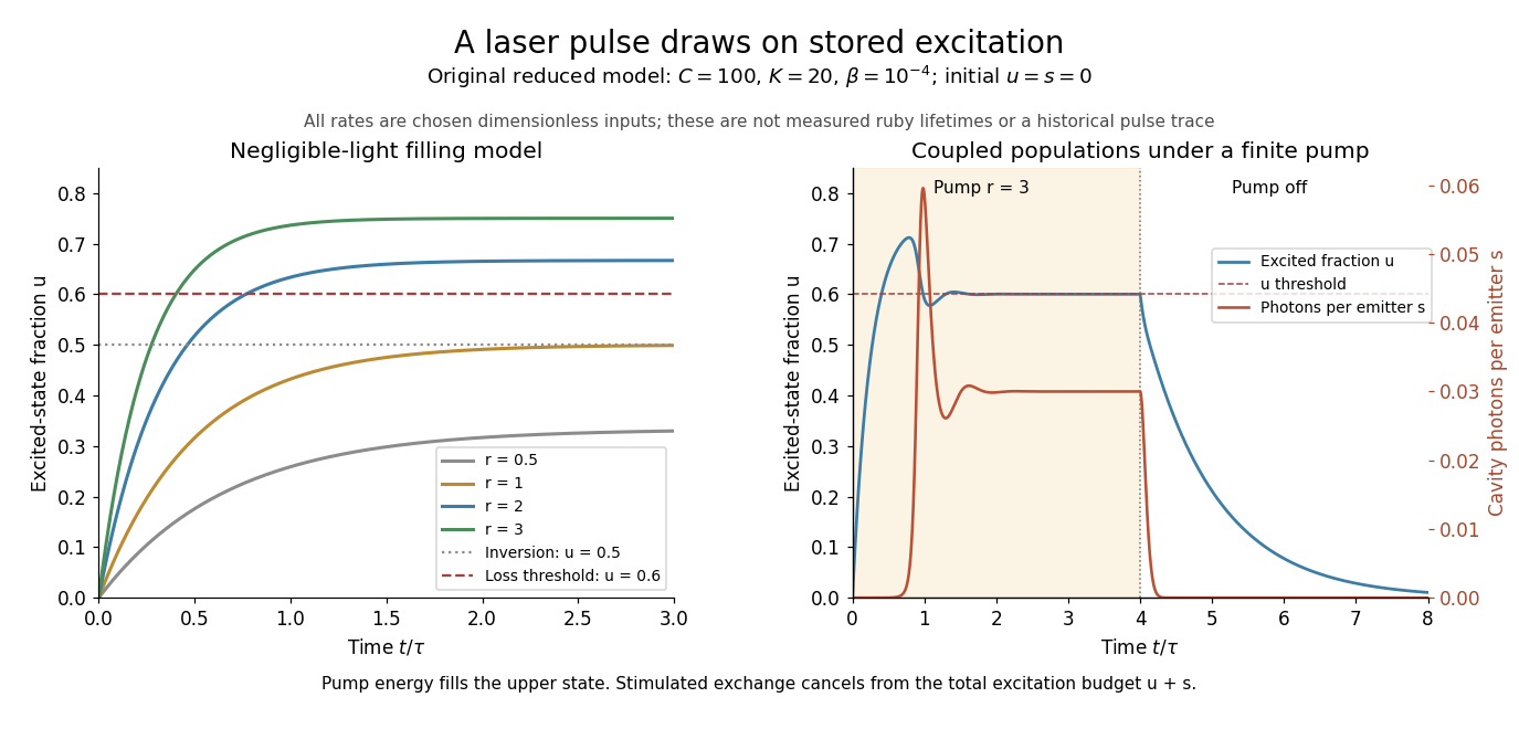
Ground-state depletion delays startup, and cavity light then drains stored excitation
. Original three-level laser rate equation calculations. Left: negligible-light upper-state fractions for several constant pumps, compared with the chosen . Right: coupled upper-state and cavity-photon populations for , , and a pump of switched off at . The rates and times are dimensionless teaching inputs, not measured ruby lifetimes or a historical pulse trace. Details.
The equations expose the excitation budget underlying conservation of energy. Adding them cancels the stimulated exchange:Pumping supplies excitations; nonlasing decay and cavity loss remove them. Integrating gives the boundOnly part of the cavity loss may be useful output; passive absorption is also a loss. The pulse's instantaneous power can draw on stored excitation, while its total extracted energy still obeys the integrated budget. The model also preserves and : at each boundary its derivatives point inward or along the boundary.
There is a further energy cost in the pump cycle. For one absorbed pump photon producing at most one emitted laser photon, the ideal energy-conversion bound isChosen wavelengths and give about before other losses. The missing energy can leave through nonradiative relaxation and heating. Actual efficiency also depends on how much pump light is absorbed, unwanted decays and optical losses; a population model alone cannot predict it.
Laser gain clamping 2026-10-18
In the steady limit with nonzero cavity light and negligible spontaneous seeding, the photon equation requires . The upper-state fraction is therefore fixed near while increased pumping principally increases the photon population. Substituting into the population equation givesFor , and , this predicts and . The inversion does not rise indefinitely above threshold. A finite supplies seed photons and smooths the ideal onset; with and exactly , the deterministic equations remain on the zero-photon solution even when that solution is unstable. This distinguishes instability of an unseeded state from actual startup of a noisy optical field.
There are unlisted articles, also show them or only show them.