
Substituting into the viscous Burgers equation gives . Integration permits the arbitrary function in the title. Multiplication of by preserves and reduces its equation to the heat equation. Thus the heat-equation representation uses a permissible time normalization rather than a condition uniquely imposed on every representative .
For a Planck function expressed as spectral radiance per frequency interval, is the Planck constant, the speed of light and the Boltzmann constant. Differentiating at fixed frequency givesThe proof uses and the chain rule. At low frequency, the multiplier tends to one, recovering the Rayleigh-Jeans law. At high frequency it grows approximately as : the same fractional temperature change has a larger fractional brightness effect on the declining spectral tail.
For an original example choose and . At , , so the first-order fractional residual is . At , , it is . Both spectra are exact blackbodies: this residual is a temperature mismatch, not evidence of a nonthermal spectrum. Fitting temperature before assessing remaining spectral residuals therefore removes a physically distinct degree of freedom. The figure divides by a fixed peak brightness rather than by the rapidly vanishing high-frequency tail.
Differential sky map monopole degeneracy 2026-10-18
An ideal differential measurement constrains two sky temperatures through . Represent every observed pair by a row of a matrix , with in column , in column and zeros elsewhere. Then and : adding any constant to the entire map changes no measurement. This null space is the angular angular monopole ambiguity, explaining why a directional comparison alone cannot measure the absolute blackbody temperature established by FIRAS.
For an original three-pixel example choose relative to an unspecified mean. Measurements and determine the third difference . The zero-mean condition recovers the chosen map, but adding to every pixel gives identical differences. The closure sum checks consistency without establishing the mean.
More generally, the graph joining measured pixel pairs must be a connected graph. If , each edge forces equal endpoint temperatures; a path propagates that equality throughout each connected component. Thus a connected observation graph leaves exactly one undetermined constant, whereas disconnected coverage leaves one per component. Fixing the mean makes an ideal connected reconstruction unique; real noise calls for least-squares solution fitting and uncertainty analysis.
The figure chooses a cosmic microwave background quadrupole sky , with and Legendre polynomial . On a great-circle scan, with measured from the chosen symmetry axis and ideal beams separated by ,Expanding proves the formula; its peak magnitude is . A constant sky gives zero. This deliberately restricted scan also misses some angular patterns, so rejecting the angular monopole is not a proof of complete sky reconstruction. Broad, overlapping coverage supplies the missing constraints; finite antenna beam patterns additionally smooth small angular features.
A hotter stellar core can favor a higher-barrier route despite fewer catalyst nuclei. To isolate this competition, prescribe a local hydrogen burning toy model at fixed mass density , with reference andChoose and , rounded barrier parameters for a proton pair and proton capture on nitrogen-14. These prescribe the temperature dependence, while the following freely chosen heating normalization incorporates effective nuclear factors and deposited energy:Here is hydrogen mass fraction, is CNO mass fraction, and is an arbitrary positive unit of stellar energy-generation rate. For and , the reference ratio is by construction. It is not a measured solar ratio. The CNO cycle bottleneck is represented by one effective rate, without evolving the existing proton-proton chain branches or catalyst network.
At , the logarithmic temperature slopes are and . The larger Coulomb barrier gives a steeper fractional response. Because these slopes change with temperature, this example retains the exponential rather than extending two fixed power laws. Writing and givesprovided the bracket is positive. With the chosen composition, . Reducing to at unchanged shifts it to . For , this catalytic route supplies no heat in this model. These are local toy crossovers: a whole star's luminosity requires integrating its stellar energy-generation rate through its stellar composition profile and stellar structure. Nuclear features, plasma screening and changes of the dominant bottleneck limit the model's extrapolation.
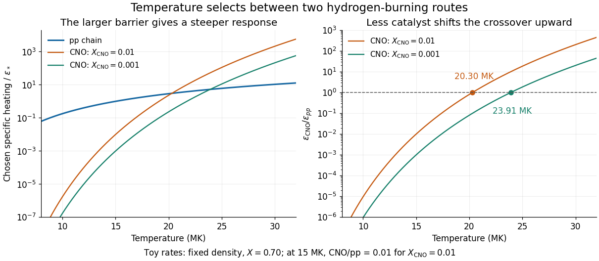
Chosen pp and CNO heating rates and their composition-dependent crossover
. Original local toy rates at fixed density and hydrogen mass fraction 0.70. The CNO-to-pp ratio at 15 MK is chosen as 0.01 for CNO mass fraction 0.01. Exponential barrier responses give crossovers at 20.30 and 23.91 MK for the two catalyst abundances. These are model curves, not stellar measurements or a fitted solar model. Details.
Isentropic decompression of a spherical linear trap Created 2026-10-18 Updated 2026-11-05
At fixed atom number, the entropy of the classical ideal gas in a spherical linear trap depends on temperature and strength through . Reversible adiabatic change therefore holds this product constant, giving the displayed relation. Reducing trap strength lowers the temperature while increasing cloud size. Its peak classical phase-space occupation remains constant, so this cooling alone does not make the gas more quantum degenerate. Heat exchange, particle loss or irreversible entropy production would change this relation.
Quantum degeneracy threshold in a spherical linear trap Created 2026-10-18 Updated 2026-11-05
For a dilute classical trapped gas, with energy zero at the potential minimum. Thus . Quantum occupation effects begin when is no longer small, giving the displayed order-of-magnitude particle threshold. Equivalently, the central density satisfies . This is a degeneracy crossover criterion rather than an exact Bose condensation threshold. In the continuum approximation, spinless bosons have excited-state saturation , from the trap density of states proportional to . A quantum ground energy should be subtracted consistently when discreteness matters.
The clamped-beam Green function is symmetric. Its explicit formula depends only on and . More generally, two integrations by parts give when at both endpoints. Applying this identity to two point-load responses shows that the displacement at one point caused by a unit force at a second equals the displacement at the second caused by a unit force at the first.
Massive-fermion chiral weight at fixed helicity Created 2026-10-18 Updated 2026-11-05
For a positive-energy Dirac spinor normalized to unit probability and with positive helicity, the left-chiral component has squared weight , where in natural units. Its right-chiral weight is ; for negative helicity the two are exchanged. In an ultrarelativistic positive-helicity particle, the left-chiral amplitude is suppressed by a mass-to-energy ratio.
Carrier density 2026-10-18
A charge carrier population per unit volume or, for a sheet, per unit area. The dimensional convention and whether different carrier species are counted separately must be specified.
X-ray fluorescence Created 2026-10-18 Updated 2026-10-20
X-ray fluorescence is Characteristic X-ray emission following excitation by incident photons. In a simple initially unexcited chemical atom, photoionization can eject an inner electron if the incident photon supplies its binding energy. An outer electron can then fill the vacancy, releasing an emitted photon with the difference of shell binding energies. Nonradiative relaxation competes with this route, so one absorbed incident photon need not yield one escaping characteristic photon.
Choose a separate stipulated electron shell model with values , and , all in . Ignore subshell splitting, recoil and changes of binding energy during relaxation. The possible shell differences areThese labels denote simplified shell groups, not resolved subshell electronic transitions. With , their calculated wavelengths are respectively , and . An incident photon exceeds both K-line energies but cannot directly create the K vacancy in this initially unexcited model. A photon can, leaving approximately of photoelectron kinetic energy. This comparison fixes neither the excitation probability nor the radiative branching probability.
X-ray emission spectroscopy Created 2026-10-18 Updated 2026-10-20
X-ray emission spectroscopy studies the frequency spectrum of emitted X-rays. The spectral line positions identify electronic energy differences; their strengths also depend on excitation, photon absorption inside the sample, geometry and detector response. An X-ray tube may excite a sample with electrons, while X-ray fluorescence uses incident photons. The distinction matters when choosing what the experiment measures: identifying a chemical element from a line position is different from determining its abundance from a line strength.
For two ideal strings under a common tension, the positive mechanical impedances satisfy , where are their linear mass densities. The reflected fraction of incident power is . Solving for the positive ratio gives or its reciprocal. Squaring yields the displayed linear mass density ratios. For , the heavier string has times the lighter string's linear mass density; the impedance ratio is only .
Reflection at a density step on a string 2026-10-18
For a massless join between two ideal strings with a common tension , require continuous transverse displacement and continuous transverse force . With for linear mass densities , the displacement reflection coefficient and transmission amplitude areThe reflected and transmitted mean-power fractions are and , with . Reflection from the heavier side reverses phase; reflection from the lighter side does not. Total reflection occurs in the limits or zero, while a finite positive impedance mismatch transmits some energy. Equal mechanical impedances remove reflection.
Viscous termination of a stretched string Created 2026-10-18 Updated 2026-10-20
A semi-infinite wave equation on a string with linear mass density , wave speed , and tension has positive characteristic mechanical impedance . At an end attached to a massless viscous damper of coefficient , displacement and transverse-force balance give the displacement reflection coefficientHere is the fraction of mean incident power dissipated. A prescribed gives two positive damper coefficients, , with opposite reflected phases. Matching removes reflection.
Degenerate-electron pressure crossover Created 2026-10-18 Updated 2026-10-20
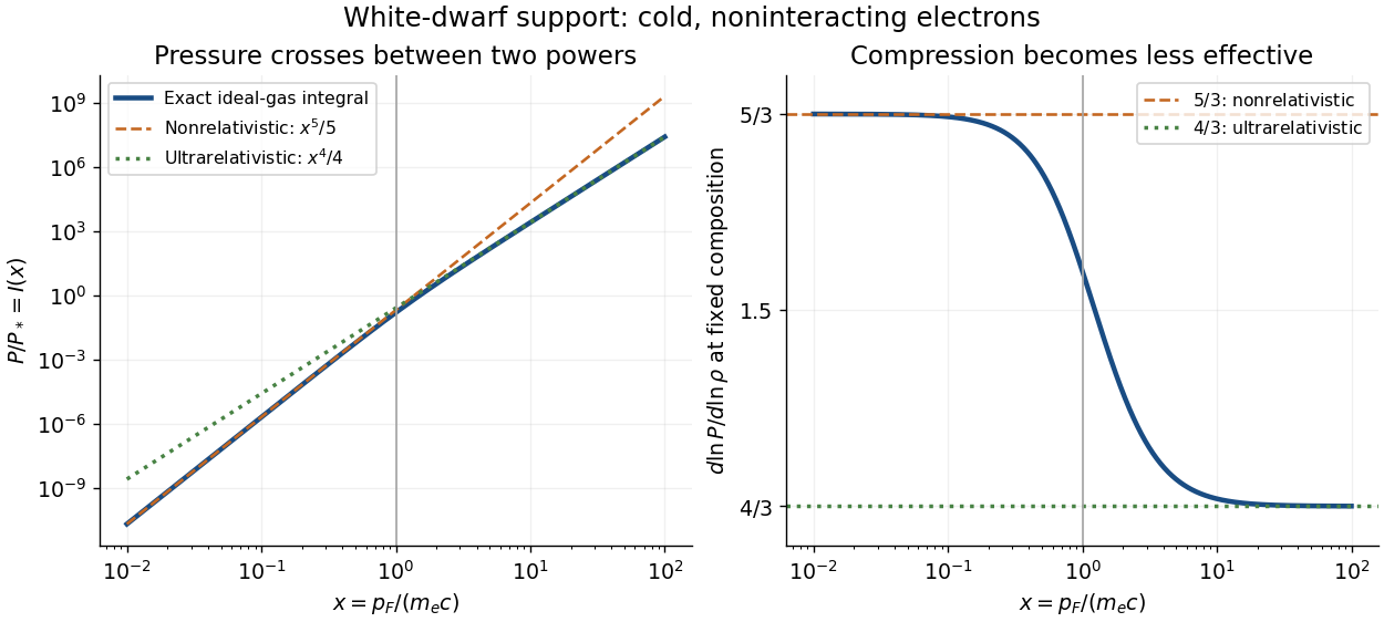
Consider an ideal degenerate electron gas at zero temperature. Counting two spin states per phase space cell gives number density . The isotropic momentum flux gives pressureHere is electron mass, is the speed of light, with Planck constant , and special relativity gives . The factor averages the directional momentum flux, and the spin factor is already included. This normalization makes a pressure, not an energy per electron.
For , expand the denominator: and . For , the integrand approaches : and . At fixed composition, mass density is , with the mean molecular weight per electron and the unified atomic mass unit. Since , the logarithmic stiffness isPressure keeps rising; its fractional gain per fractional compression becomes smaller. Relativistic electrons approach a speed ceiling while their momenta keep increasing. Thus the high-density equation of state loses the extra compression leverage of a nonrelativistic white dwarf. The Chandrasekhar mass from central polytropic constants supplies the corresponding global mass calculation.
For a calculated local example with , gives , and . Its stiffness is , intermediate between the two limits. These are ideal equation of state values at one point, not a measured central mass density or a whole white dwarf model. Finite temperature and interactions are excluded.

For a real skew-symmetric matrix , is invertible: would imply . Its Cayley transform is an orthogonal matrix, since transposition gives and the commuting factors cancel in . Also , so in every dimension. If , then . For , the transformed eigenvalue is . In odd dimension , so has a nonzero kernel and fixes that direction.
Cayley's matrix memoir 2026-10-18
Arthur Cayley's 1858 paper A Memoir on the Theory of Matrices motivates matrices as an abbreviated way to write systems of linear equations. Its opening already connects the characteristic equation with reducing polynomials in a matrix to lower degree. In §21 he works out the two-by-two identity; in §23 he says he has verified the three-by-three case but does not give a formal proof for every size. Thus this source distinguishes the general statement from a general proof.[ref]
A Memoir on the Theory of Matrices by Arthur Cayley. Printed pp. 17–18, opening motivation; pp. 23–24, §§21–25, characteristic equation and reduction of matrix functions; received 10 December 1857, read 14 January 1858, published 1858
The theorem's name also commemorates William Rowan Hamilton.Take a different real matrix,Its only eigenvalue is , with algebraic multiplicity two. However, the polynomial , which vanishes at that eigenvalue, gives . Merely checking values at eigenvalues cannot prove a matrix identity. The full characteristic polynomial does work:The matrix is a Jordan block, and its minimal polynomial is also .
The binomial theorem gives, for positive integers ,Terms containing or a higher matrix power vanish. After removing the common growth factor , the remaining linear map is the shear mapping . It moves to . The single eigenvalue controls the exponential scale, while the nilpotent matrix adds a factor growing linearly in .
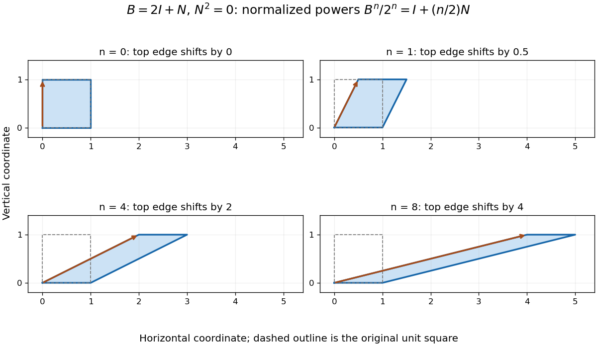
Normalized powers of a Jordan block retain a growing shear despite having only one eigenvalue; equal axes scales show the top edge moving by n/2
. Details. 
In terms of polynomial interpolation, reduction modulo retains both a value and a derivative:Indeed, polynomial division gives . This is a simple Hermite interpolation condition. For , it gives exactly the displayed matrix power. Repeated eigenvalues retain information about how a polynomial changes, not just where it vanishes.
Polynomial reduction of matrix powers 2026-10-18
By polynomial division, write with . Because is a monic polynomial, this division works even over a commutative ring. Evaluating at makes the multiple of vanish, leaving . This explains the reduction in two-coefficient reduction of matrix powers without multiplying out every intermediate matrix.
Over a field, the minimal polynomial divides and gives the strongest such universal reduction: use the polynomial remainder modulo instead. For the scalar matrix , the characteristic polynomial is , while the minimal polynomial is only . Every matrix power is then a scalar multiple of .
Two-coefficient reduction of matrix powers 2026-10-18
Consider the real matrixThe Cayley-Hamilton theorem gives . ConsequentlyThusAll four entries come from just two scalar coefficients. If , multiplying once by and replacing gives the linear recurrence relationEquivalently , with . The appearance of Fibonacci numbers is explained by , where advances the Fibonacci recurrence. No eigenvectors need to be computed.
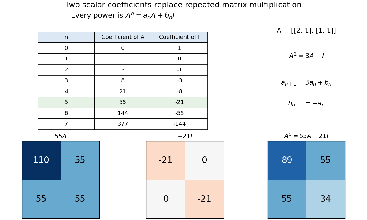
Cayley–Hamilton reduces powers of a chosen two-by-two matrix to two integer coefficients; the fifth power is 55A − 21I
. Details. 
The same identity computes an inverse. Rearrange it as , givingThis works because the constant term of this characteristic polynomial is nonzero and the coefficients lie in a field. Generally, when over a field, rearranging the Cayley-Hamilton theorem expresses as a polynomial evaluated at a matrix. Over a general commutative ring, a nonzero constant need not be a unit; invertibility requires that extra condition.
There are unlisted articles, also show them or only show them.