
Torsional measurement of a complex shear modulus Created 2026-10-18 Updated 2026-10-20
A thin uniform circular rod of radius and length undergoing a small end twist of complex amplitude has shear-strain amplitude . A complex viscoelastic modulus gives shear-stress amplitude . Integrating the restoring torque givesThe area integral is the polar second moment of the cross-section, not a mass moment of inertia. For a disc of moment of inertia and negligible rod inertia, harmonic angular motion satisfies in a free-mode calculation, or equals the external torque amplitude in a driven measurement. The complex stiffness is a frequency-domain constitutive representation; a general real-time response has memory and cannot be described by putting an arbitrary frequency-dependent complex number into an instantaneous real equation.
For a localized quantum harmonic oscillator along , let the transverse magnetic vector potential be for , with zero potential before the switch. The Coulomb gauge form of minimal coupling gives . The creation operator matrix element means that only is reached at first order from the ground state. Its interaction picture amplitude isIn particular , so resonant finite-time expressions are nonsingular. The induced electric dipole moment is . It contains a driven component with the dynamic electric polarizability and free-frequency transients required by the initial conditions. The discontinuity in gives an impulsive electric field and an initial mechanical velocity even though the initial canonical momentum has zero mean.
Dual norm supremum need not be attained 2026-10-18
On the real space of sequences converging to zero , use the supremum norm and define the linear functionalThe geometric series gives , so is a bounded linear functional and . The sequence with its first entries equal to one and all later entries zero belongs to , has unit supremum norm, and gives . Hence . But if and , not all coordinates can equal one or all equal minus one. Since every weight is positive, . The supremum is approached but never attained on the unit ball.
Dual norm as a worst-case linear error bound 2026-10-18
Suppose a perturbation satisfies , with . Absolute homogeneity of a norm and the dual norm definition giveFor nonzero , divide it by its norm to obtain an input in the unit ball; for zero perturbation the inequality is immediate. This is an exact error bound for a linear functional, for every perturbation in the stated input set.
For and a budget , the sharp output-error bounds are for , for , and for . Scale the maximizing vectors from the preceding example by to attain the positive endpoints; their negatives attain the negative endpoints. The L1 norm budget constrains a total absolute error; the maximum norm budget permits each coordinate to have that error separately. These budgets define nested sets and carry different information.
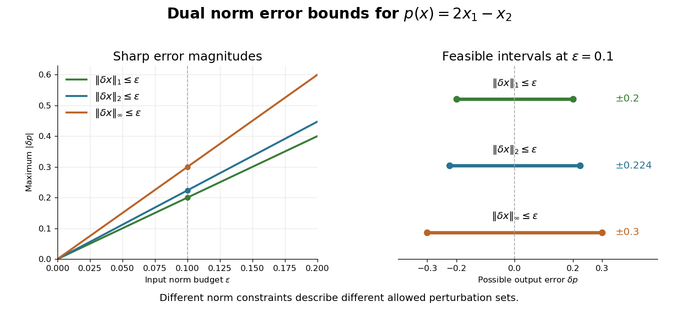
Dual norms give exact worst-case errors for the same linear functional
. Original bounds for . Lines show the sharp error magnitude as the stated input norm budget increases. The right panel gives the full possible error intervals at ; these are the full feasible intervals for the stated deterministic bounds. Details.The coordinates must use the stated scale and units. Rescaling one coordinate changes both its coefficient in and the meaning of its input budget. For a nonlinear differentiable function with scalar values, its Fréchet derivative at the base point is a linear functional governing the first-order response. An exact finite-perturbation error bound additionally needs control of the Taylor remainder or of the Fréchet derivative along the path.
Phase-reversed double-slit diffraction Created 2026-10-18 Updated 2026-10-20
Two equal rectangular apertures of width , centre spacing , and relative phase have Fraunhofer diffraction amplitude proportional to , with and . HenceThe interference zeros satisfy , including the central dark fringe. The single-aperture envelope vanishes at for nonzero integer . A uniform phase reversal translates the narrow-slit fringes by half a fringe without changing their spacing.
Keplerian radial-velocity curve 2026-10-18
A repeating Doppler shift contains more than an amplitude. For an isolated two-body problem, let be the true anomaly, the stellar argument of periapsis, the periapsis time and the constant system line-of-sight velocity. The companion's argument of periapsis differs by from , so mixing the two conventions reverses the orbital signal. With positive velocity for recession, choose the stellar line-of-sight coordinate positive away from the observer. Kepler's equation supplies the clock:Here is the mean anomaly and the eccentric anomaly. The time coordinate is uniform in , not in : an eccentric Kepler orbit runs fastest near periapsis.
To derive the velocity law without guessing a sinusoid, write the stellar orbital coordinates as and . Project toDifferentiating and substituting the true anomaly identities givesThe constant term makes the time average of the orbital velocity zero: returns to its original value after one orbital period. For this reduces to a sinusoid with an arbitrary phase origin; periapsis itself is then undefined. For , the largest and smallest velocities are , so is still half the peak-to-peak range, although the extrema need not be symmetric about .
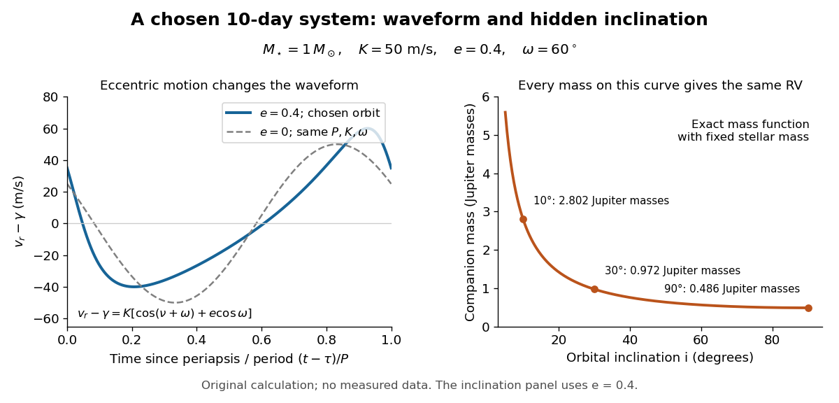
For an original worked example, choose , days, , and . Taking one day as and , the binary mass function is . Its units check directly: . With adopted solar mass and Jupiter mass , solving the exact binary mass function gives
| Orbital inclination | Companion mass |
|---|
All three systems have the same chosen and therefore the same Doppler spectroscopy time series, despite different true masses. Exactly what remains fixed is ; alone is only the small-companion approximation. The value is the minimum mass. For this example the extrema are and relative to , and the periapsis value is . This is a chosen eccentric system, not a reconstruction of 51 Pegasi b.


Discovery of 51 Pegasi b 2026-10-18
Michel Mayor and Didier Queloz began observing 51 Pegasi in September 1994 and revisited its repeating Doppler spectroscopy signal in 1995. Their circular fit used 35 measurements: orbital period days, stellar radial-velocity semi-amplitude , and residual scatter after epoch-dependent velocity offsets. Apparently stable comparison stars checked the instrumental zero point. Low chromospheric stellar activity and an inferred roughly 30-day stellar rotation period argued against starspots; light curves and the spectral line bisector tested stellar pulsation. These checks favoured orbital motion but had finite sensitivity. The reported Jupiter masses was not a true mass. Stronger upper bounds used stellar-spin information and assumed spin–orbit alignment, limiting a nearly face-on binary star interpretation conditionally.[ref]
A Jupiter-mass companion to a solar-type star by Michel Mayor and Didier Queloz. Mayor and Queloz (1995), pp. 356–358, figures 2–4, table 1, and alternative interpretations; scan: wwelsh.sdsu.edu/CLASSES/ASTR510/PAPERS/Mayor-Queloz_51Peg.pdf
The hot Jupiter matters both for planetary migration and for how exoplanets are found. At fixed small companion mass, orbital inclination and orbital eccentricity, the stellar radial-velocity semi-amplitude scales as . Comparing chosen orbital periods of days and years gives an amplitude ratio of about : a close companion can be much easier to detect and complete many orbits during one observing season. Finding a giant planet close to its star also asks how its present orbit relates to where it formed. Doppler spectroscopy supplies a dynamical constraint; it does not by itself establish a formation pathway or measure the exoplanet's radius.
ELODIE spectrograph 2026-10-18
Built by André Baranne, Michel Mayor, Didier Queloz and colleagues, the ELODIE fiber-fed spectrograph carried light from Haute-Provence's 1.93-metre telescope through optical fibers. Its echelle grating dispersed light in high diffraction orders; an optical prism and grism cross-disperser separated them perpendicularly on a charge-coupled device. This cross-dispersed echelle spectrograph achieved spectral resolving power . A simultaneous thorium reference tracked instrumental drift. Wavelength calibration mapped detector positions to wavelengths; spectral cross-correlation combined many spectral lines into a fitted profile. A barycentric velocity correction removed the observer's motion.[ref]
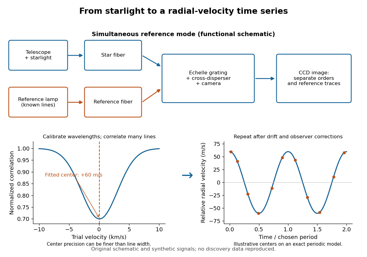
ELODIE measurement chain and synthetic radial-velocity readout
. Original schematic; the correlation profile and periodic signal are synthetic. Details.
Why can a spectrograph measure a Doppler shift much smaller than one spectral resolution element? Resolution concerns separating neighbouring features, whereas locating the centre of a known profile uses information across that profile and across many spectral lines. For a chosen example, at a recession velocity of givesAt , one spectral resolution element corresponds to , about times larger. A well measured centre can move by a small fraction of that width. More photons and more useful spectral lines improve the estimate, but do not remove wavelength calibration errors or stellar activity.
A simple mathematical picture of spectral cross-correlation makes the readout concrete. Define , with fixed reference wavelength , and let be continuum-normalized line absorption. For small velocities, a common Doppler shift approximately translates . A positive absorption mask then givesIf , the maximum occurs at ; a convention correlating the received observed radiative flux instead produces a dip. A fitted correlation centre is an effective collective line position, not a claim that each individual spectral line has been resolved into a narrower feature. The lamp tracks instrumental drift, while the barycentric velocity correction removes the observer's changing line-of-sight velocity; neither removes changes in the star itself.
Barycentric velocity correction Created 2026-10-18 Updated 2026-10-20
The correction for an observer's motion relative to the Solar System barycenter along the target line of sight. Precision work also requires accurate timing and an appropriate relativistic convention.
Symmetry of divided differences 2026-10-18
A divided difference depends on the chosen interpolation nodes and their data, but is unchanged by any permutation of those same interpolation nodes. The explicit sum in divided difference makes this visible: a permutation merely rearranges its summands.[ref]
There is also a short explanation using Lagrange cardinal polynomials. The coefficient of in the th Lagrange cardinal polynomial is . Taking that coefficient in their weighted sum gives exactly the explicit divided difference formula. Since polynomial interpolation has a unique answer for a fixed set of distinct interpolation nodes, this coefficient cannot depend on their ordering. If the interpolation polynomial has polynomial degree below , the coefficient is zero.
For the four-point example in divided difference table, every ordering gives third divided difference . This does not make every Newton polynomial coefficient invariant: whereas , because these use different pairs of interpolation nodes. Even at second order, and use different triples. The node order in Newton interpolation determines which subsets occur along the top row.
Divided difference table 2026-10-18
A divided difference table arranges divided differences by starting interpolation node and order . Its base column is ; every later entry uses two neighboring entries from the previous column:The denominator spans all interpolation nodes of that entry, even though the numerator uses adjacent table entries. The interpolation nodes must be distinct; they need not be equally spaced or sorted.[ref]
3.3 Interpolation. NIST Digital Library of Mathematical Functions; §3.3(iii), equation 3.3.34: initial values and divided-difference recurrence for distinct nodes
Take the polynomial at the interpolation nodes , giving values . Its divided difference table isThe first divided differences are , , and . The second divided differences use the wider spans: and . The third divided difference is . Reading the top row gives the Newton polynomial coefficients , rather than all the entries in any one column.
The resulting Newton polynomial grows through four partial interpolants:At , misses by ; the correction supplies exactly there and vanishes at the earlier interpolation nodes . At , misses by ; the correction supplies exactly there and vanishes at all three earlier interpolation nodes. Each added term therefore preserves the previous agreements while satisfying the next one.
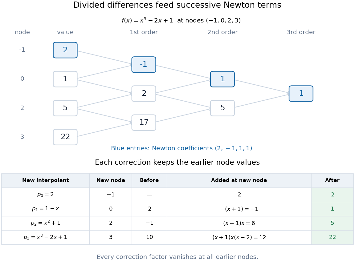
Divided-difference triangle and successive Newton interpolants for the constructed polynomial x cubed minus 2x plus 1
. Details. 
For interpolation nodes, the triangle contains recurrence steps. Once the top row is known, nested evaluation of the Newton polynomial uses only multiplications and additions per argument. The triangle organizes the work; the factors explain why the construction works.
For distinct points , the cross product in the numerator has magnitude twice the area of the triangle with third vertex . The same double area is the base length times the perpendicular height from , proving the displayed Euclidean distance. Equivalently, let and project onto the line direction. The squared distance is ; Lagrange's identity gives the same cross-product formula.
Dirty image 2026-10-18
The dirty image is the direct weighted inverse Fourier transform of the measured complex visibilities:The final equality follows by substituting the point-source complex visibility and exchanging the finite sums. For continuous brightness it is a convolution with the dirty beam, with the primary beam included in the brightness when necessary. Negative values and subsidiary peaks can arise from that response even when every true source has positive strength.
For on , impose zero Dirichlet boundary conditions on the two vertical sides and the top, and a zero Neumann boundary condition at the bottom. The Dirichlet gauge transform for constant drift gives . Separation of variables produces the displayed modes, with and . Their spatial parts are orthogonal with weight ; equivalently, expand in the ordinary sine-cosine basis.
For the forward diffusion equation on , with and homogeneous Dirichlet boundary conditions, a solution continuous on the closed initial-boundary domain can take initial data only if . These equalities express the same corner value through the initial condition and the boundary condition.
An incompatible endpoint value does not prevent an interior or L2 space initial-data solution. For example, on the initial ramp givesIt satisfies both zero endpoint values for every and tends to at every fixed as , also in the L2 norm. It cannot extend continuously to with both the initial value one and the boundary value zero. Each sine term vanishes at the endpoint, so the series cannot silently repair that pointwise contradiction.
If the equation is written , the intended forward heat coefficient requires . For , the ramp's coefficients would grow like , failing square summability for every . This example distinguishes an incompatible corner from the separate ill-posedness of backward diffusion.
Cyclotron mass in a graphene cone Created 2026-10-18 Updated 2026-10-20
A massless-cone description permits a nonzero cyclotron effective mass. For a circular constant-energy contour of area , the semiclassical definition givesThe vanishing mass parameter in a Dirac Hamiltonian and the finite cyclotron response away from neutrality are different statements. This makes the temperature dependence of Shubnikov-de Haas oscillations a useful test of the dispersion rather than a measurement of an electron's vacuum rest mass.
Carrier density in a graphene cone Created 2026-10-18 Updated 2026-10-20
Assume zero temperature, the linear Dirac cone, and both real-spin states and both electronic valleys. Define as excess electron number per unit area, negative for an excess of electron holes, relative to neutrality. A filled circular region of radius in wave vector space containsThus the excess carrier density grows quadratically with the Fermi energy, unlike the constant density of states of a parabolic two-dimensional band. Differentiating gives the positive density of states per unit area, . Both the geometry of occupied states and the fourfold degeneracy matter to the coefficient.
Sublattice pseudospin in graphene 2026-10-18
At and positive energy, a normalized eigenvector for is . Its Pauli matrix expectation values give the displayed direction. This pseudospin records the relative amplitudes and phase on the two sublattices. Real spin supplies another label; confusing these two labels would double-count states and misinterpret the two-band Hamiltonian.
Dirac point Created 2026-10-18 Updated 2026-11-05
A Dirac point is a momentum-space point where two energy bands touch and their leading splitting is linear in displacement from that point. A local two-band Hamiltonian often takes the form , where is measured from the touching point and the Pauli matrices act on a two-component internal basis.
Its energy eigenvalues are , producing a Dirac cone. The two components can label sublattices rather than real spin. Adding a symmetry-allowed term opens a gap , illustrating why the symmetries protecting the touching matter. Distinct Dirac valleys in graphene are regions around different Dirac points.
Extracting a semiconductor band gap from diode saturation current Created 2026-10-18 Updated 2026-11-05
In a diffusion-dominated p-n junction, with a transport prefactor determined by minority-carrier diffusion and dopant densities. Combining this with the intrinsic carrier concentration gives, for fixed gap and effective masses,The slope against is . A measured diode ideality factor helps identify the transport regime: generation or recombination current can have a different dependence on , so its activation slope cannot automatically be interpreted with the diffusion formula.
There are unlisted articles, also show them or only show them.