
Mean squared displacement Created 2026-10-18 Updated 2026-10-25
A mean squared displacement is the expected value of a squared position change over a specified time lag. For isotropic free diffusion in dimensions, it equals . A nonzero mean drift contributes its squared displacement as well as the displacement variance; specifying the tracked coordinates and whether the mean is subtracted is essential.
Fair sampling 2026-10-18
For a specified Bell test statistic, fair sampling assumes that conditioning on successful detections preserves the correlations needed to represent the intended ensemble. Constant detector efficiency in an independently specified loss model can ensure this; constant observed count rates alone do not establish independence from the hidden state. The Polarization CHSH count model explicitly assumes independent losses.
If genuine pairs arrive at rate before the timing cut, an exposure gives and expected accidental pairs . In a background-dominated large-count approximation, maximizing reduces to maximizing for . Differentiation gives the positive stationary solution , or . The endpoint solves the rearranged equation but is outside the domain of this derivative calculation; tends to zero at both positive-domain extremes.
Thus the chosen gives for this particular criterion, accepting about of genuine delayed signals. This differs from maximizing signal counts alone, which would favor longer windows. Small samples, appreciable signal fluctuations, unknown background, dead time and multiple-candidate vetoes require a fuller likelihood model. The calculation isolates a tradeoff rather than prescribing an experimental cut.
Connect every pair among moving scalar coordinates and one fixed coordinate by identical springs of stiffness . The coupling pattern is the complete graph with one vertex fixed. Its potential energy is . The moving-coordinate stiffness matrix is the principal submatrix displayed in the header. For equal masses , the uniform normal mode has squared angular frequency , while every sum-zero vector has squared angular frequency . There are such degenerate modes. This follows directly from the Laplacian spectrum of a complete graph and its rank-one matrix form. Constant gravitational forces shift the equilibrium without changing the stiffness.
Area and length of a cycloid arch 2026-10-18
For the cycloid , , , , the area between the arch and its baseline isIts arc length isThe positive sign of inside this parameter interval removes the absolute value in the speed. Omitting the two endpoint cusps does not change either integral.
Crystal basis structure factor Created 2026-10-18 Updated 2026-11-05
The crystal basis structure factor is the coherent sum of scattering contributions from the atomic basis of a crystal at a chosen reciprocal lattice vector :The positions lie within a cell and are the corresponding scattering amplitudes. Fractional coordinates give .
The Bravais lattice sum fixes possible Bragg-peak positions, while this basis sum controls their amplitudes and can cancel some exactly. Two identical sites separated by half a cubic body diagonal give a factor , extinguishing odd sums. Replacing one site by a different species generally prevents that cancellation. The intensity involves , so amplitudes must be added before squaring.
Single crystal Created 2026-10-18 Updated 2026-11-05
A single crystal is a crystalline specimen whose ordered structure has one continuous crystallographic orientation, rather than being divided into differently oriented crystal grains. It can still contain dislocations, impurities and other defects; the term does not mean an absolutely perfect lattice.
A diffraction pattern from one well-oriented specimen resolves its crystallographic directions, while rotating it changes which reflections are observed. Mechanical or thermal measurements along different directions can reveal intrinsic anisotropy that would be averaged over many orientations in a polycrystalline material. The absence of internal grain boundaries also changes transport and deformation mechanisms that depend on those boundaries. A specimen's outline is not the criterion: cutting a piece from a single crystal changes its external shape without necessarily changing its internal crystallographic identity.
For a fixed unit vector , the linear map has kernel and image the perpendicular plane . Thus is solvable exactly when , and then its full solution set isFor the proof, a cross product with must be perpendicular to . Conversely the vector triple product identity gives , which determines the perpendicular orthogonal projection of . The remaining parallel component is arbitrary. Finally when , verifying sufficiency.
Geometrically, the solution set is a straight line with direction . Its nearest point to the origin is and its distance from the origin is . For a general nonzero fixed vector , the corresponding formula is , again subject to .
For a unit vector , real , and real , the displayed linear equation has the unique vector solutionTo prove it, split vectors into components parallel and orthogonal to . On the parallel line, the linear map is multiplication by . On the perpendicular plane, the operator obeys , by the vector triple product. Therefore on that plane. Combining its inverse with the parallel solution gives the formula. This avoids component calculations in equations with an axial cross product term.
A mass-spring-damper subject to a constant load obeys at critical damping. With and ,For , the displacement exceeds its final value at a positive time exactly when . Thus a critically damped step response released from rest is non-overshooting, but critical damping alone does not forbid overshoot from arbitrary initial momentum. For a vertical scale with downward coordinate, and , making the threshold .
Energy balance of coupled RL circuits 2026-10-18
The magnetic energy of this constant-inductance model isThe positive-definite matrix condition makes . Multiplying the two circuit equations by and , then adding, gives the displayed conservation of energy statement: input power supplies stored magnetic energy and Joule heating. With zero drive, . After the drive becomes zero, the stored magnetic energy supplies the remaining Joule heating.
Apply for and then set the drive to zero while retaining the closed primary return. By superposition, each pulse-response electric current is its equal-loop RL induction step response at minus that response at , with the step response defined as zero before its onset. All currents remain continuous at ; the drive changes their derivatives.
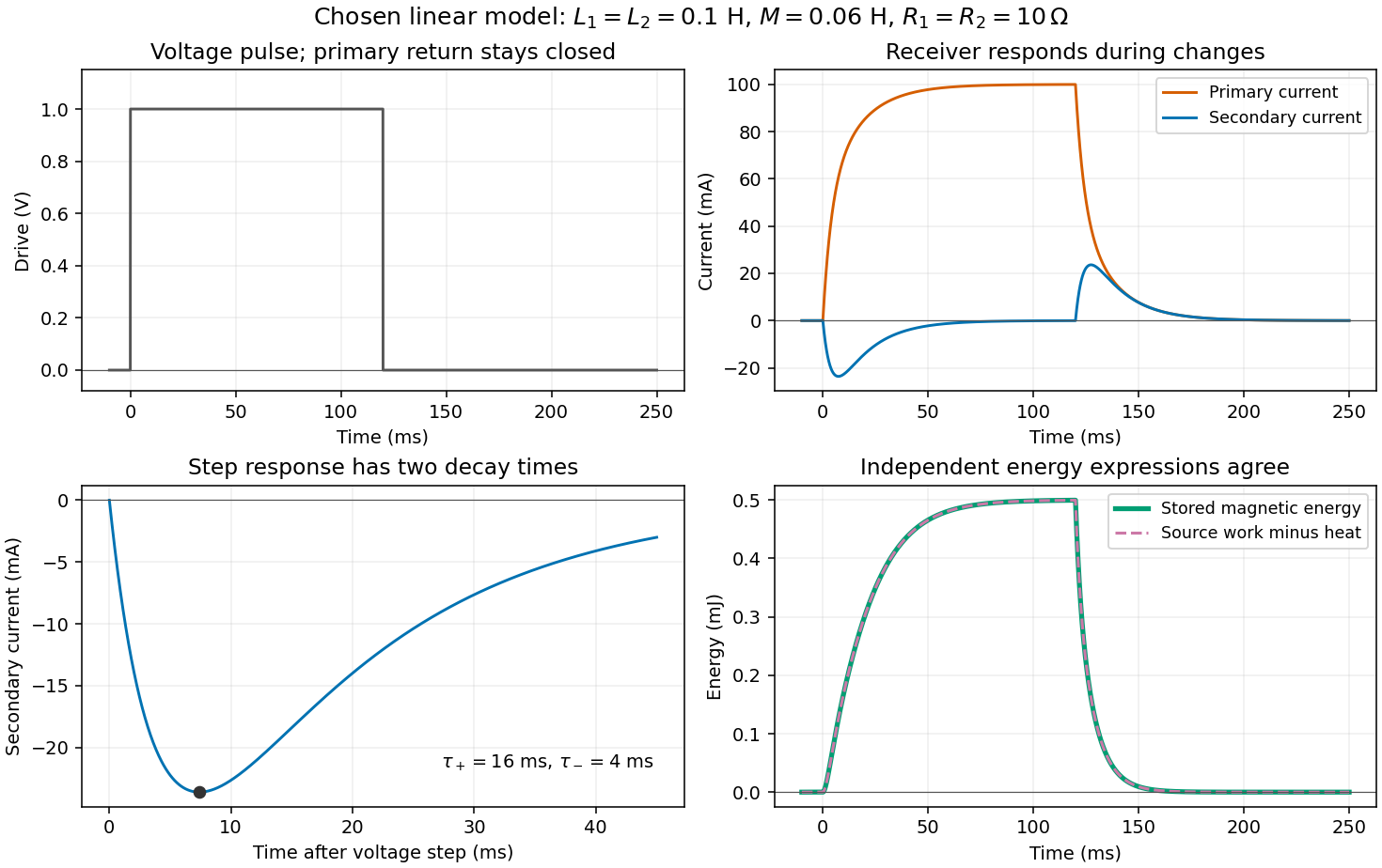

For the displayed pulse, the secondary responds negatively as the primary builds and positively as it decays. Between these transients, the primary is almost steady and the secondary is almost quiet. The energy balance of coupled RL circuits accounts for the entire process, including the energy remaining in the magnetic field when the drive changes.
Equal-loop RL induction step 2026-10-18
For an exactly soluble example, set , , and . Start with zero electric currents, and apply a constant electric potential difference at . The sums and obey separate first-order linear differential equations:Their time constants are and . Thus, for ,Since , for , but as . The primary approaches . The secondary response opposes the rise of linked magnetic flux, in accordance with Lenz's law. Removing mutual inductance by setting makes the two exponentials equal and gives zero secondary electric current.
For stipulated , , and , the two time constants are and . Setting gives its largest negative magnitude atThe continuing primary electric current eventually reaches while the secondary returns to zero. These numbers belong to the stated model, not the 1831 apparatus.
Hess cosmic-ray balloon experiment 2026-10-18
Victor Franz Hess's 1912 series used two sealed, 3-mm-walled ionization chambers with Theodor Wulf's fiber electrometers. Karl Bergwitz suggested internal plating; Günther & Tegetmeyer improved focusing. Basket-mounted ground comparisons, insulation-loss measurements, simultaneous detectors and barograph-derived heights supplied checks. The highest flight reached 5350 m; its comparisons came from Vienna and after landing, without a launch-site baseline.[ref]
Über Beobachtungen der durchdringenden Strahlung bei sieben Freiballonfahrten by Victor Franz Hess. 1912, pp.1084-1085 apparatus and preparations; pp.1087-1088 seventh flight; English primary-text translation arxiv.org/pdf/1808.02927 pp.1-2, 5-6
A third, thin-walled chamber admitted ambient air. Hess multiplied its readings by , with pressure in millimeters of mercury, warning that vessel-wall contributions might violate this scaling. He recorded outside temperature but applied no absolute-temperature correction. Night flights, an eclipse and weather observations constrained alternatives to radiation from above; the eclipse argument addressed directly propagating solar radiation.[ref]
Über Beobachtungen der durchdringenden Strahlung bei sieben Freiballonfahrten by Victor Franz Hess. 1912, p.1085 pressure reduction; p.1086 eclipse; p.1088 temperature footnote; pp.1090-1091 inference; English translation pp.2-3, 6-8
The electrometers read gradual electric potential loss caused by continuing air ionization. The low-altitude dip and strong high-altitude rise favored an extraterrestrial contribution, without measuring proton composition.[ref]
Über Beobachtungen der durchdringenden Strahlung bei sieben Freiballonfahrten by Victor Franz Hess. 1912, pp.1089-1091 altitude averages and interpretation; English translation pp.7-8
An ionization chamber integrates electric charge: one energetic particle may create many ion pairs, several particles may contribute to one reading, and a photon can create charged particles in the gas or walls. A voltage-loss reading is therefore neither a count of primary cosmic rays nor a chemical analysis of them.Domenico Pacini supplied independent evidence: in June 1911 he compared a copper-box-enclosed electroscope at the sea surface and 3 m underwater, more than 300 m offshore above an 8-m-deep seabed. Reduced underwater ionization, stable electrical loss between runs, and a lake comparison supported an external contribution independent of soil radioactive decay. Water provided shielding; this established a different constraint from Hess's altitude comparison.[ref]
La radiazione penetrante alla superficie ed in seno alle acque by Domenico Pacini. Pacini's 1912 report, English translation pp.3-5, especially surface/underwater comparison and residual-ionization discussion; original Italian facsimile pp.9-14
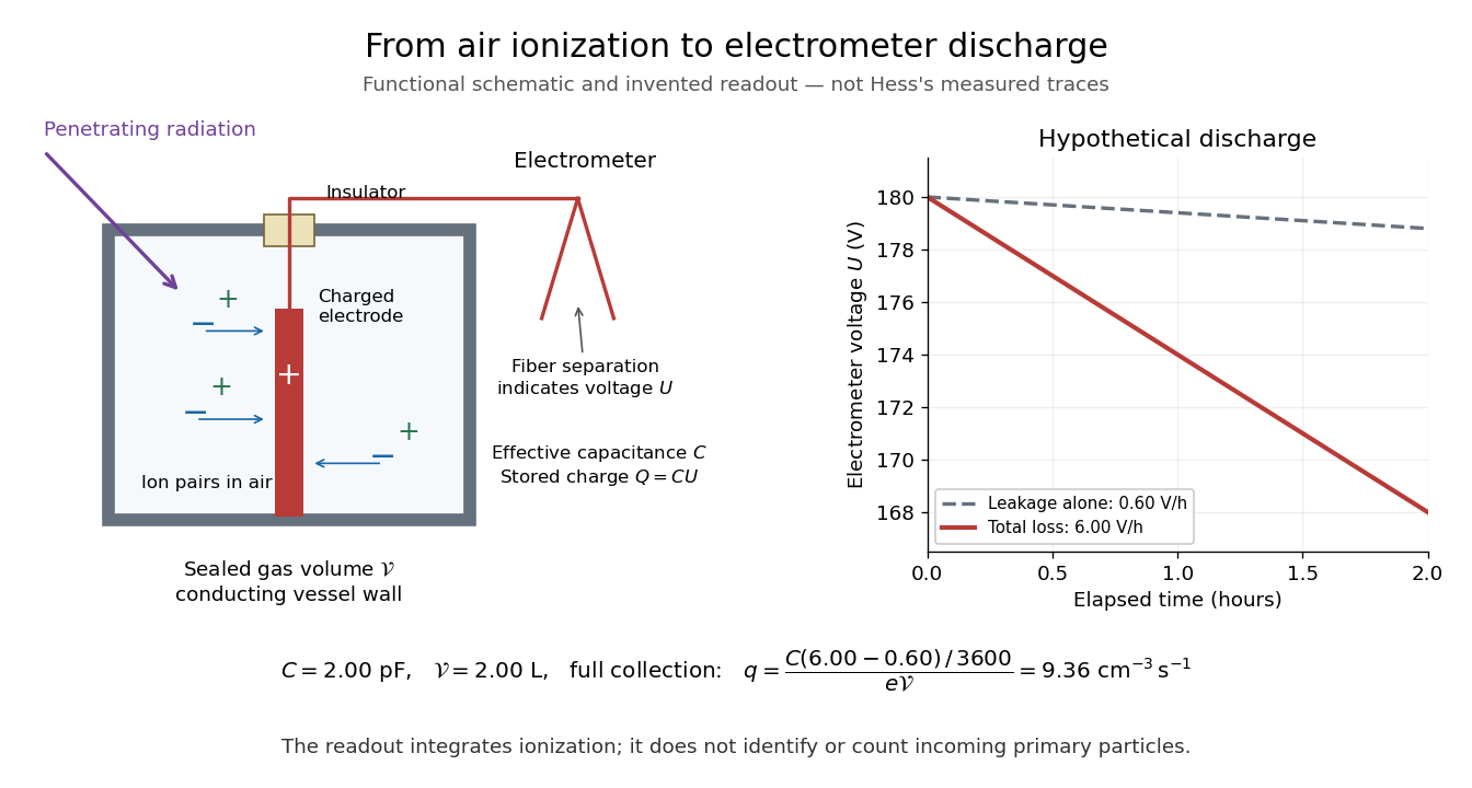
From air ionization to electrometer discharge
. Original functional schematic and invented readout example for the ionization-chamber charge-loss model. The chamber drawing is not a dimensional reconstruction, and the plotted voltage traces are not Hess's measurements. Details.
Air shower 2026-10-18
An air shower is a cascade of secondary particles produced by an energetic particle interacting in the atmosphere. Both a charged particle and a gamma ray can start one.[ref]
Cosmic Rays: Particles from Outer Space by CERN. A new world of particles, secondary showers; Cosmic accelerators, gamma-ray showers
Secondary cosmic ray 2026-10-18
A secondary cosmic ray here is a particle produced by an atmospheric interaction of a primary cosmic ray or its descendants. A muon at ground level need not have traveled from the original astronomical source.
Primary cosmic ray Created 2026-10-18 Updated 2026-10-20
Convolution of a Cauchy distribution and a uniform distribution Created 2026-10-18 Updated 2026-10-20
Let have the Standard Cauchy distribution and let , independently, have the uniform distribution on , where . The convolution of probability densities gives the probability density of asThis is an even function. Its derivative isso its unique mode is zero. Its tails satisfy as : multiplying the integral by makes the integrand converge uniformly to on the bounded interval . Consequently both positive and negative parts of the first moment diverge, so its expected value does not exist. The symmetric Cauchy principal value of that moment is zero, which is a different assertion. Adding a bounded independent displacement smooths the probability density without removing the divergent first moment of the Cauchy distribution.
BCS dimensionless coupling 2026-10-18
Use for the normal-state single-spin density of states per unit energy and volume at the Fermi surface. Write the attraction as , with , and define .[ref]
Theory of Superconductivity by John Bardeen and others. p.1182, equations (2.34)–(2.40), one-spin density of states; volume normalization stated here
Since has units of energy, has units of energy times volume, making dimensionless. Set , an energy cutoff using the Debye frequency , rather than a frequency itself. These conventions also fix the meaning of the earlier constant-shell BCS gap equation.
Here is the reduction of the BCS gap equation in these conventions. Substituting the zero-temperature BCS anomalous average givesThe sum counts one spin species. For , cancelling and replacing this sum by an integral with constant givesThe factor two from the symmetric integral cancels the in the BCS anomalous average; it is not an extra spin degeneracy. Substituting evaluates the integral as . Solving givesThe first equality is exact within the constant-density of states, sharp-cutoff mean-field approximation; the last is the weak coupling asymptote. Extending the first equality to large does not make this simplified model an accurate description of a strongly coupled material.
For an original numerical example, choose and . The exact constant-shell BCS gap equation gives ; the weak coupling formula gives . Its fractional underestimate, measured against the exact result, is exactly . At that error is , so the two formulas are no longer interchangeable. No material parameters have been fitted here.
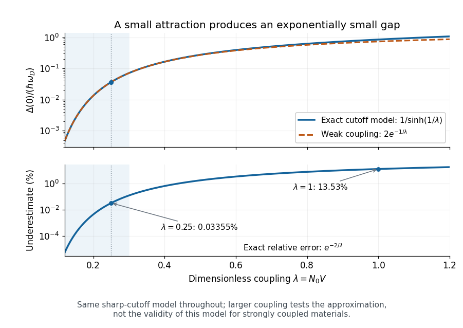
The exact cutoff gap and the range of the weak-coupling approximation
. Original zero-temperature constant-shell BCS gap equation calculation. The upper panel compares with ; the lower panel gives the exact fractional underestimate . The shaded interval is a chosen small-coupling illustration, not an experimental boundary. The large-coupling part tests the asymptote within the same model. Details.
At nonzero temperature, substitute the finite-temperature BCS anomalous average instead. The same cancellation yieldsAt the superconducting transition temperature take the continuous limit. The integrand at then has the finite limiting value , so no divergent endpoint needs to be inserted into a numerical quadrature. For , the resulting integral gives and . These ratios concern the isotropic weak coupling model.[ref]
Microscopic Quantum Interference Effects in the Theory of Superconductivity by Leon Neil Cooper. 1972 lecture, thermodynamic properties of the ideal superconductor, pp.80–82
Tiny-pivot roundoff in Gaussian elimination 2026-10-18
A nonzero pivot element can still be a poor numerical choice. Partial pivoting bounds the absolute values of the elimination multipliers by one in exact arithmetic, because each numerator is no larger than the selected denominator. This usually improves numerical stability, but does not prevent every possible growth of intermediate entries or guarantee accurate answers for every linear system.[ref]
2.6 Row pivoting. Fundamentals of Numerical Computation by Tobin A. Driscoll and others; §2.6.4, Example 2.6.6, equation (2.6.3) and concluding discussion: small-pivot instability and the limits of pivoting
To see the mechanism without depending on hardware, define a toy floating-point arithmetic model. The operator rounds an exact real number to the nearest value with three significant decimal digits; halfway cases choose the even final digit, and . Allow an unbounded exponent range. Round the inputs and the result of every addition, subtraction, multiplication and division separately; a product followed by a subtraction rounds twice. This is a prescribed arithmetic model, not a measurement of a physical computer. All inputs in the following original example are represented exactly:Without a row interchange, the elimination multiplier is . The last coefficient and right-hand side becomeTwo distinct exact values now have the same rounded representation. Back substitution therefore returnsThe small difference carrying information about was lost during elimination; the final subtraction only exposes that loss. Dividing by the tiny pivot element amplifies sensitivity to the lost information.
With partial pivoting, interchange the two rows, including their right-hand sides, to start from . Now , and the rounded updates areBack substitution gives and . Both paths round intermediate values, but only the first creates million-sized entries and then divides a lost difference by .
The true solution follows from the original second equation :Evaluate the linear-system residual against the original data in exact arithmetic, separately from the three-digit solve. With , the maximum norm, the results areThe respective relative linear-system residuals are and . Computing the diagnostic in higher precision matters: a check made only against the rounded reduced equations would miss the original error.
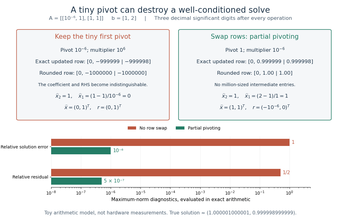
The same three-digit floating-point arithmetic model gives without a row interchange and with partial pivoting; exact linear-system residuals expose the difference
. Details. 
This matrix is well conditioned in the maximum norm: its induced matrix norm is , whileThe failure therefore belongs to this unpivoted algorithm, rather than a large condition number. In general, however, partial pivoting cannot remove sensitivity inherent in the data. For any approximate solution of an invertible matrix system, ; the induced matrix norm inequality and giveA small linear-system residual controls solution error only in conjunction with the condition number; numerical stability and sensitivity are different questions.[ref]
There are unlisted articles, also show them or only show them.