
Symmetric part of an orthogonal matrix 2026-10-18
For a real orthogonal matrix , . If for a nonzero complex eigenvector, then . Therefore the same eigenvector has eigenvalue for the symmetric part of a matrix . Orthogonality implies , so writing gives . The complete complex orthonormal eigenbasis of an orthogonal matrix shows that all the eigenvalues of its symmetric part lie in .
Normal subgroups and quotients of the symmetric group on three letters Created 2026-10-18 Updated 2026-10-20
The conjugacy classes of the symmetric group on three letters have sizes : the identity, the three transpositions and the two 3-cycles. A normal subgroup is a union of whole conjugacy classes and contains the identity. Its candidate orders are therefore . Lagrange's theorem excludes four, leaving precisely , and . The order-three subgroup is the cyclic group of the two 3-cycles and the identity; it is also the kernel of a group homomorphism of the sign map.
The first isomorphism theorem gives the corresponding quotients , and the trivial group. Thus these are exactly the possible images of surjective group homomorphisms from . Each occurs, by the identity map, the sign map and the constant identity map, respectively.
Suppose are bounded functions on the same nonempty set, and the supremum norm of their difference is at most . Then their optimal values differ by at most the same amount:Indeed, for every , so ; exchange and for the other direction. Adding a constant shifts a supremum by that constant, a basic compatibility between upper bounds and addition.[ref]
For a chosen example on , take and . Their supremum error is , since . Completing the square givesThus has maximum zero at , while has maximum at . The change in optimal value, , is smaller than the certified bound . For the vertical translation , the bound is exact: its supremum error and optimal-value change are both .
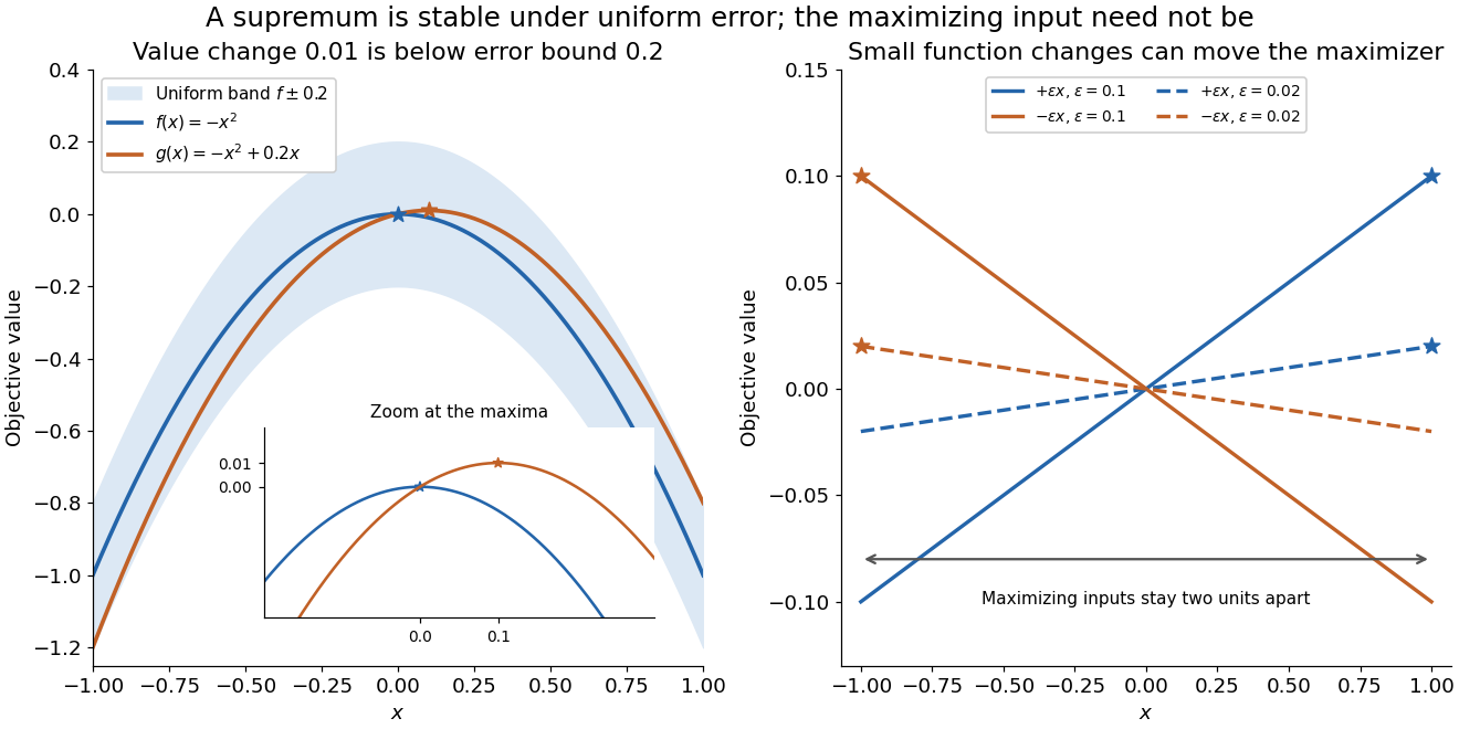
Uniform error controls the optimal value; maximizing inputs require additional control
. Original polynomial examples on . Left: and lie within a vertical error band of , while their maxima differ by . Right: the small tilts and have maximizing inputs and for every ; solid lines use and dashed lines use . These chosen examples are not measured errors or claims about an arbitrary optimizer. Details.
A stable optimal value does not guarantee a stable maximizing input. On , the two linear functions and satisfyFor every positive , their unique maximizing inputs remain two units apart, at and . Both functions approach the flat zero function, which has many maximizing inputs. Consequently an accurate objective function value is not by itself a certificate that the optimizing decision is accurate.
The estimate also gives a convenient consequence of uniform convergence. If converges uniformly to a bounded function on a nonempty , then for the bounded tail of the sequence. Uniform control handles the changing input that defines the best value. Pointwise convergence alone supplies no such control; the existing examples under uniform convergence illustrate that distinction.
Supremum of a sum 2026-10-18
Let be nonempty sets of real numbers bounded above. Their Minkowski sum is , allowing every pair from the Cartesian product . ThenThe sum of the two suprema is an upper bound for every permitted sum. For the reverse bound, use the approximation property of a supremum to choose and . Their sum is within of the claimed value. This reasoning does not require either supremum to be a maximum.
Separate choices matter. On , choose the functions and . Each has supremum one, but their sum at a shared input is always one:The maximum of occurs at , while that of occurs at . A common input cannot realize both choices. With separate inputs, choosing and gives . The allowed pairs of output values are the entire unit square for separate inputs, but only the line segment for the shared input.
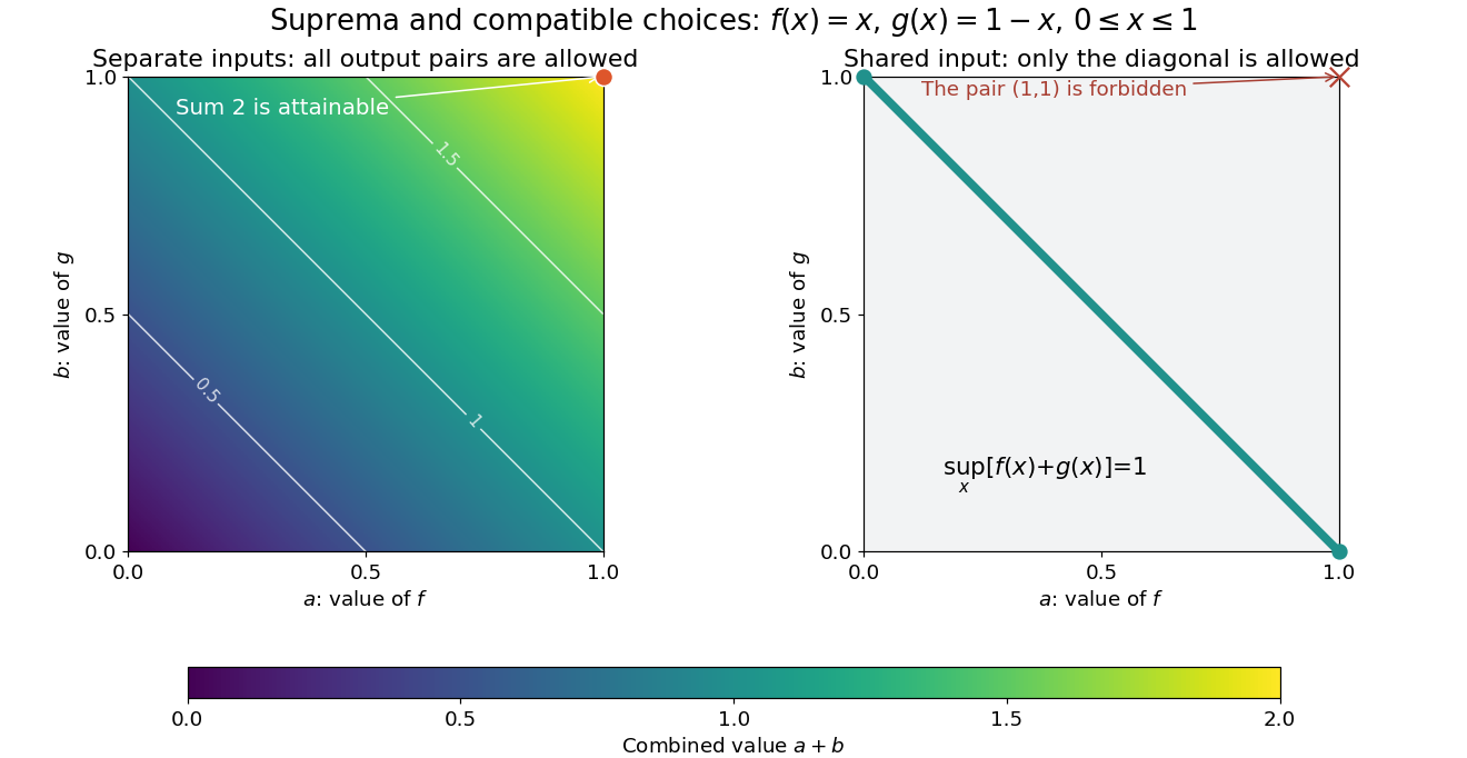

For any two bounded functions on the same nonempty domain of a function, the useful general estimate isThe inequality can be strict, as the example shows. Equality does not require attained maxima, but it does require that the two large values can be approached at compatible inputs. For example, on gives equality with value two, although neither function reaches its supremum. This distinction is useful when an objective function combines terms sharing a decision variable: adding the best possible termwise scores gives an upper bound, not necessarily a feasible combined score.
Low-redshift acceleration cosmography 2026-10-18
A local derivation makes the acceleration sign transparent. Normalize and put . A Taylor series givesThe radial null geodesic in FLRW spacetime gives . Invert the redshift series, use through second order, and obtain the displayed luminosity distance. Spatial curvature of an FLRW universe first changes this relation at third order. Lower therefore means larger at a fixed sufficiently small positive redshift and common .
Worked supernova distance comparison 2026-10-18
Stipulate and , so . A megaparsec is parsecs. Neglect radiation in cosmology. Compare an accelerating flat model , an open matter-only model and the Einstein-de Sitter universe . Their present deceleration parameters are respectively , and . For these models,Here is dimensionless; the radial null geodesic in FLRW spacetime supplies its integral and spatial curvature of an FLRW universe supplies . The observer-to-source comoving radial distance is , whereas the transverse distance uses . Omitting the latter distinction would bias the open-model comparison.
At , numerical integration gives for the flat accelerating model and for the open matter-only model. ThusThe accelerating model is mag fainter than the open matter-only prediction at the same redshift and standardized absolute magnitude, corresponding to times the luminosity distance and times the radiative flux. These are model calculations, not observations from either collaboration.
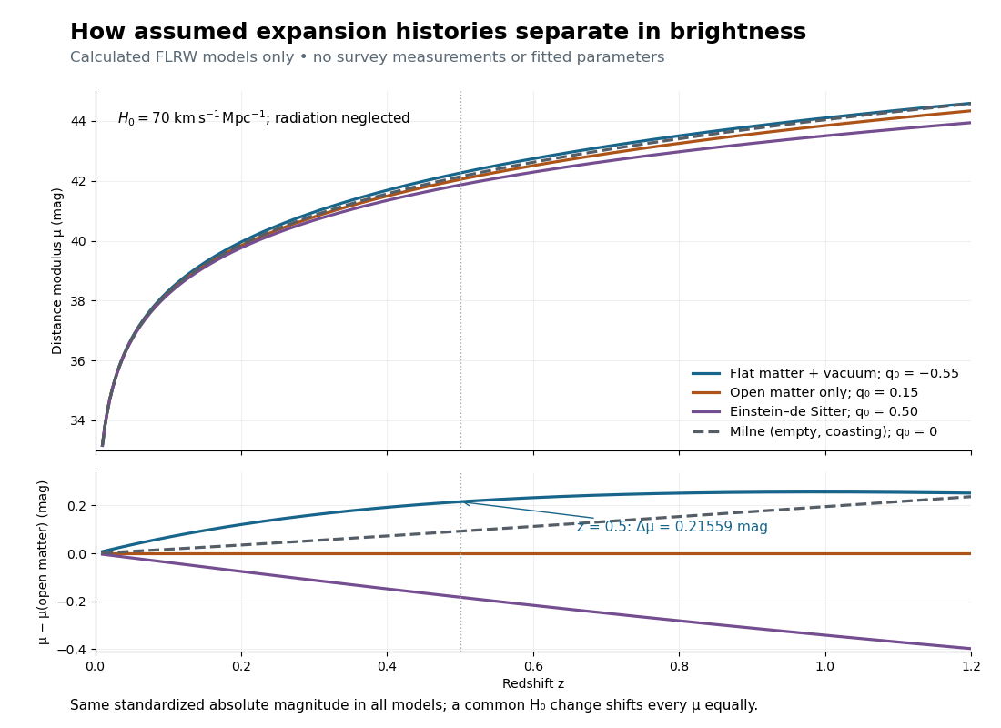

The Milne model has , and , giving and . The Einstein-de Sitter luminosity-distance relation independently checks the flat matter-only integral. At , the accelerating model exceeds the Milne model by only mag, illustrating the dependence of a residual on the chosen reference. Over a longer redshift interval, luminosity distance integrates past deceleration as well as recent acceleration; a residual need not increase forever.
Multiplying by at fixed density fractions divides every by and shifts every distance modulus by . The predicted apparent magnitude is unchanged if simultaneously increases by . This is the absolute magnitude–Hubble constant degeneracy. For example, shifts by mag and by mag. Relative curves at the same retain their separation; determining requires an external absolute magnitude calibration.
Supernova Cosmology Project Created 2026-10-18 Updated 2026-11-05
The Supernova Cosmology Project measured the brightness-redshift relation of Type Ia supernovae to constrain matter density and the contribution represented by a cosmological constant. Its high-redshift sample was fitted together with nearby events after standardizing peak brightness using light-curve information.[ref]
Measurements of Omega and Lambda from 42 High-Redshift Supernovae by Saul Perlmutter and others. Abstract: distant/nearby samples, standardization and joint cosmological fit
Its importance includes an independent observing and analysis effort alongside the High-Z Supernova Search Team. Independence of teams does not eliminate all shared uncertainty: both rely on related supernova physics, nearby calibration and assumptions connecting luminosity distance with an expansion model.
High-Z Supernova Search Team Created 2026-10-18 Updated 2026-11-05
The High-Z Supernova Search Team used distant Type Ia supernovae to compare the observed relation between luminosity distance and redshift with models of cosmic expansion. Its analysis combined distant events with nearby calibrators and tested how light-curve fitting and sample choices affected the inferred acceleration.[ref]
Observational Evidence from Supernovae for an Accelerating Universe and a Cosmological Constant by Adam Riess and others. Abstract: nearby/high-redshift samples, fitting methods and systematic tests
The physical inference is that sources at a specified redshift were farther away than predicted by relevant nonaccelerating comparison models. Calibration, extinction and population evolution are therefore central to interpreting the brightness difference, rather than secondary corrections to an otherwise direct acceleration measurement.
The current-phase relation of a superconducting weak link gives its pair electric current as a function of the Gauge-invariant Josephson phase , at specified temperature and other conditions. For the ideal junction used below, with . More general periodic relations can contain higher Fourier harmonics; their maximum magnitude defines the corresponding superconducting critical current.
Abrikosov vortex 2026-10-18
An Abrikosov vortex has a core where the superconducting order parameter is suppressed, surrounding circulating electric currents, and a winding of its quantum phase. A singly wound vortex carries one superconducting flux quantum in the appropriate bulk flux-quantization limit. The exact contour statement is fluxoid and flux quantization in a superconductor; the enclosed magnetic flux alone need not equal a flux quantum on a contour with appreciable electric current.
Super-Kamiokande atmospheric-neutrino experiment Created 2026-10-18 Updated 2026-10-20
Super-Kamiokande used days ( kiloton-years) and fiducial kilotons of water. Inner photomultiplier times and charges reconstructed interactions; the outer anticoincidence detector vetoed entering particles and marked exits. Contained single-ring events used likelihood classification: electron particle showers blur rings; muons give sharper edges. The visible-energy sample division is not a universal detection threshold. Simulation estimated classification efficiency above about , distinct from total detection efficiency; stopping muons and decay electrons checked classification.[ref]
Evidence for oscillation of atmospheric neutrinos by Y. Fukuda and others. PDF pp. 2–3, Table I: apparatus and classification
Downward neutrinos travel about ; upward ones about . The multi-GeV muon-like up/down asymmetry was ; electron-like events lacked a comparable effect. Calibration constrained directional bias. This was disappearance evidence; tau neutrino appearance was untagged and sterile conversion remained possible.[ref]
Writing and for the selected upward and downward populations, the asymmetry is : a negative value means fewer upward events. An absolute source-normalization error alone rescales both populations and leaves this ratio unchanged. A direction-dependent response error need not cancel.
Neutrino-flux sensitivity inversion 2026-10-18
Why compare inferred neutrino fluxes rather than raw event counts? For channel , exposure time , target population , cross section , and detection efficiency including reconstruction and selection, a forward model isHere is expected background; on the left counts events, while counts targets. Distinct cross sections, target numbers, thresholds and detection efficiencies prevent a direct CC/NC count ratio from being an electron neutrino fraction. Channel populations themselves can be correlated estimates from overlapping event patterns.
An original reduced linear algebra model isolates the inference. Assume specified spectral shapes and divide each background-corrected channel rate by its own calibrated electron neutrino response. Put and let be the spectrum- and response-weighted non-electron/electron ES sensitivity ratio. ThenThe equal and responses determine their sum, not their separate neutrino fluxes. Changing the assumed spectra generally changes the integrated coefficients; with arbitrary unknown spectra this small matrix is insufficient.
Choose illustrative inputs, not historical measurements: , and , with every neutrino flux in the same arbitrary unit. The forward prediction is . CC and NC independently invert to , ; substituting into ES returns . Alternatively, CC and ES give . Thus the third channel tests the response model and the inferred mixture.
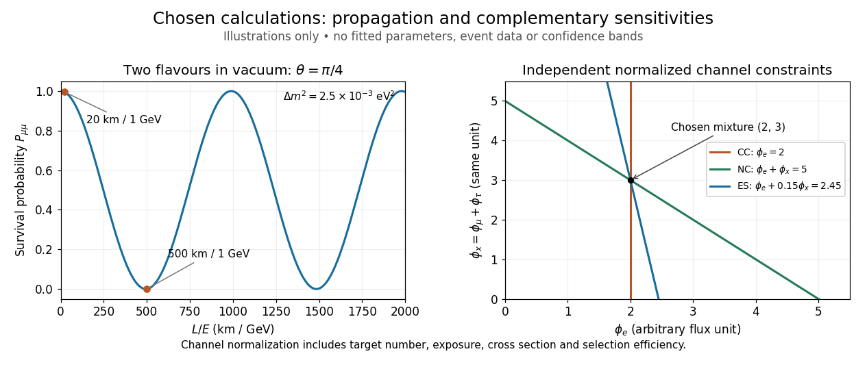

CC alone admits any nonnegative . CC and ES lose the second independent constraint when ; for small positive , an ES-minus-CC error is amplified by . With chosen independent errors , their propagated standard deviation is . If CC and NC instead have those independent errors, the difference has standard deviation . Actual analyses must retain covariances, including those introduced by statistical channel separation. Complementarity supplies information; calibration establishes what information each channel carries.
SNO solar-neutrino flavor experiment Created 2026-10-18 Updated 2026-10-20
In 2001, live days, reconstructed radius below and effective electron kinetic energy above gave a CC neutrino flux of for the assumed boron-8 spectrum. Source calibrations measured instrumental-cut signal loss. SNO's own CC–ES difference was ; comparison with Super-Kamiokande's precise ES flux gave evidence for non-electron active neutrinos. This was not an NC measurement.[ref]
In 2002 the pure-heavy water analysis used live days and a reconstructed kinetic-energy threshold. NC neutrons captured on deuterons emitted gamma rays, producing secondary electron light. The NC reaction threshold was , a different quantity. Californium-252 calibrated capture efficiency, but only detection efficiency after fiducial and energy cuts. Assays constrained backgrounds from radioactive decay and photodisintegration.[ref]
Direct Evidence for Neutrino Flavor Transformation from Neutral-Current Interactions in the Sudbury Neutrino Observatory by Q. R. Ahmad and others. PDF pp. 2–3: neutron calibration, thresholds and backgrounds
Energy, radius and direction relative to the Sun statistically separated channels. Assuming the standard boron-8 spectral shape, the NC total active neutrino flux was , consistent with stellar structure predictions. The non-electron active component differed from zero by . This established active flavour conversion, without individually tagging muon neutrinos and tau neutrinos. It did not exclude every sterile admixture.[ref]
A steady spherical subsonic isothermal breeze with isothermal sound speed obeys . Since , its finite-radius speed maximum lies at . Spherical mass conservation then gives the displayed density, where is the peak Mach number. This free parameter is selected by a boundary condition, not by , and alone. Therefore , while a peak Mach number of order unity gives that expression as a characteristic scale.
A direct demonstration of the free parameter comes from the first integral . Its additive constant remains free for a breeze; imposing the regular transonic branch would be a different condition.
For unattenuated isotropic radiation from a point source, the radiation pressure force on each absorbing particle is . Dividing by its mass changes the effective inverse-square inward acceleration to . The wind equation therefore places the maximum of a subsonic isothermal breeze at the displayed radius, provided the bracket is positive. If it is nonpositive, the positive-temperature subsonic outflow decreases in speed throughout its domain and has no interior speed maximum. A cross section per particle requires that particle's mass; an opacity per unit mass instead absorbs this conversion.
Trivial subgroup Created 2026-10-18 Updated 2026-11-05
Subgroup test 2026-10-18
A nonempty subset of a group is a subgroup if and only if for every . Necessity follows from closure and the existence of inverse elements in a subgroup.
Conversely, choose . Setting gives the identity element . Taking then gives for every . Finally, using as the second element gives , proving closure. The inherited multiplication is associative, so these properties establish the group axioms on .
For and zero endpoint values, write with , and . The change of variable has and sends , . Thus it is an isometry from the weighted inner product to the ordinary integral on , and the apparent singular operator becomes . Its Dirichlet eigenvalues are and its normalized eigenfunctions are , . The singular endpoint is handled through this transformed regular domain; a zero eigenvalue occurs exactly when .
Nonpositive modes in a Dirichlet-Robin interval expansion Created 2026-10-18 Updated 2026-10-31
For , positive eigenvalues have eigenfunctions , where and . Their squared norms are . A zero eigenvalue occurs precisely at , with eigenfunction . A negative eigenvalue occurs precisely at : it is with eigenfunction , where . There is exactly one such , since decreases strictly from to . The integration by parts identityand the Cauchy-Schwarz inequality show positivity for and nonnegativity at equality. The complete expansion of a square-integrable function therefore includes the extra term when , or when , in addition to . Omitting that extra mode makes the system incomplete. In particular, at is orthogonal to every positive sine mode and is an immediate counterexample to a sine-only expansion.
Strong induction and accumulated hypotheses 2026-10-18
Strong induction does not prove more than ordinary mathematical induction. Put . Ordinary mathematical induction on retains the earlier cases and obtains the next one, establishing the same conclusion. Conversely, an ordinary inductive step can ignore the extra cases allowed in a strong induction hypothesis.[ref]
Mathematics for Computer Science by Eric Lehman and others. §5.3, printed pp. 129–130: equivalence of induction formats and well ordering
The well-ordering principle gives another view. A least counterexample would have all smaller cases true, so the strong induction step would establish that allegedly false case. The starting case excludes the beginning.
There are unlisted articles, also show them or only show them.