The surface tension has dimensions , while and . ConsequentlyMatching the dimension of height gives , so . Dimensional analysis fixes this exponent but cannot determine a dimensionless prefactor or a contact-angle dependence.
Using the convention , the series RLC circuit has complex impedanceAt the stated frequency, and . ThusThe vector is in the resistance–reactance plane. Positive reactance means that the net circuit is inductive and current lags voltage. With the alternative convention the imaginary signs reverse, while the magnitude and physical phase relationship agree.
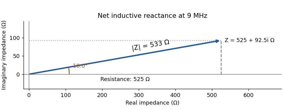
Series-circuit impedance in the resistance–reactance plane
. Details. The string's no-slip condition gives . Conservation of mechanical energy from release to the stated height drop yieldsSolving for the spool's moment of inertia,The axle does no work because its point of application is fixed, and the ideal string and axle introduce no losses. The spool mass is not needed to infer from this energy measurement.
The slit spacing is . At normal incidence, the diffraction grating maxima satisfy . ThereforeThe third order would require , so it cannot propagate. At fixed order and spacing, a longer wavelength requires larger . Green light has a larger first-order diffraction angle than blue light.
At closest approach the velocity is tangential. The conserved specific orbital energy and specific angular momentum areThe negative energy gives an elliptic orbit. Its semi-major axis isSince ,This treats the star as fixed, appropriate to . Equivalently, equate the energy at the two turning points using . The planet mass cancels; a circular-orbit relation would be inappropriate here.
After the push, the forces are weight downward, normal reaction upward and sliding friction opposite the velocity. There is no continuing applied push. The table has constant slopeVertical balance gives , and horizontal motion gives . ThusThe friction magnitude is .
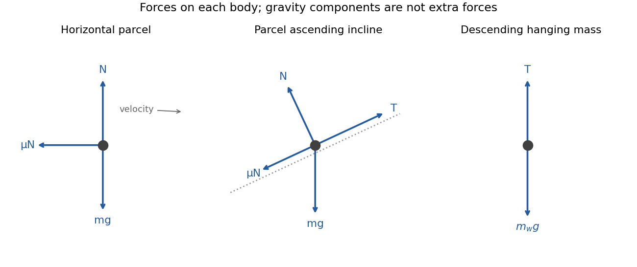
Free-body diagrams for horizontal sliding, the inclined parcel and the hanging weight
. Details. The inclined parcel has tension up the slope, weight vertically downward, normal reaction and friction down the slope. The hanging mass has weight downward and tension upward. The ideal string makes the two acceleration magnitudes equal.
The velocity slope is , up the track for the parcel and downward for the hanging mass. The free-body diagrams show gravity itself as one vector; its slope-parallel and normal components are used in the equations rather than counted as additional forces.
Let and let be the hanging mass. Taking up-slope and downward respectively as positive,Eliminate the common tension to obtainHere , and . The pulley changes the direction of the string force; in the ideal model it does not change its magnitude.
The required constant deceleration follows from :Both gravity and sliding friction oppose ascent, so . WriteThe physical incline solution is more precisely . The combined mass cancels from the equation. The top of the track is consequently above its base.
Let be the compression and the combined mass. Starting from rest at the top, it falls through before maximum compression. HenceThe gravitational drop during compression must be included. Equating to the weight would instead describe a static equilibrium, not the turning point after a fall.
Immediately after the parcel leaves, the spring still stores , but only the sledge is launched. Choose gravitational potential zero at the ramp base. Its initial position is , so conservation of energy to the apex givesThereforeabove the ramp base. Its upward travel from the compressed position is , a different distance from the height above the base.
For actual complete bounce distances and , the geometric series givesA natural intended estimate compares the observed first round trip with the loss-free round trip from the initially compressed position,If the reduction factor is taken to be , the answer is . The first term is the actual 4 m, not the hypothetical loss-free distance.
This numerical inference needs the stated comparison assumption. Strictly, knowing the first actual bounce distance and saying subsequent distances share a ratio does not independently specify that ratio. A change in spring compression also means that an energy-loss fraction is not automatically the same as a vertical-distance ratio.
The collinear relativistic velocity addition formula isWith both velocities directed toward Earth,The denominator keeps the result below . Adding the two speeds by the Galilean rule would give an inadmissible .
The separation simultaneous in the mothership frame at launch is the length contraction of the Earth-frame simultaneous separation:In that frame Earth approaches the launch position at while the lander travels toward Earth at . Their coordinate separation closes at , soA closing rate between two objects can exceed ; it is not either object's speed in the other's rest frame. Simultaneity matters: simply transforming the Earth event at Earth-frame launch time would not give the simultaneous mothership-frame separation.
For the lander, , soThe relativistic kinetic energy isThe rest energy is excluded from kinetic energy.
Set the launch event to and measure toward Earth in light-years and in years, so light has coordinate slope magnitude one. Earth's worldline is , and the lander's is . The outgoing signal is and reaches Earth at . Earth's reply is sent at .
The return signal has . Its intersection with the lander gives . Both signal lines are null; the lander's worldline lies inside the light cone. The drawing exaggerates the small gap near Earth in an inset so that B, C and D remain distinguishable.
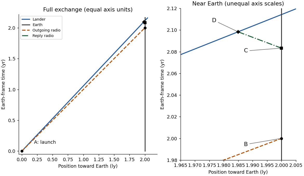
Equating the lander and return-signal positions givesThis is measured from launch, so about 25.18 months pass on Earth-frame synchronized clocks. D occurs slightly before the lander reaches Earth at .
The two events A and D lie on the inertial lander's own worldline, and their proper time difference isEquivalently, applying the Lorentz transformation with gives .
The central rod occupies the holes in the discs, so the disc masses must be annular rather than counted as solid discs overlapping the rod. Define . ThenThe axial moment of inertia isThus , exactly the axial inertia of a uniform disc of outer radius and mass . The cancellation uses the given density–length relation.
The contact radius is , so rolling without slipping gives . With , the energy at the minimum of the stated parabolic motion model isConsequentlyThe corresponding spin angular frequency is . It is the rod radius, not the disc radius, that relates translation and rotation; the discs determine the larger rotational inertia.
In the small-amplitude approximation, is the speed along the track, and supplies the gravitational potential. The conserved energy isDifferentiating and extending through turning points by continuity givesThis is simple harmonic motion with . HenceThe frequency is lower than for a sliding point mass because energy is also stored in rotation.
For weak linear damping, write the amplitude envelope as . The amplitude e-folding time is , and one period is approximately . ThusEnergy, being proportional to amplitude squared, decays twice as rapidly in its exponent. Using its e-folding time instead would introduce a factor-of-two error.
At the initial turning point the oscillation energy is . In the high-quality factor regime, , so the required input per period isThis replaces the small dissipated energy each cycle, rather than supplying the entire stored energy again.
is the particle's potential energy as a function of position, and is its total energy eigenvalue in this time-independent Schrödinger equation. Solving it with the boundary conditions determines the allowed stationary states and energy levels.
The wavefunction is a probability amplitude: the Born rule gives position probability density , normalized to unit integral for one particle. itself need not be real or positive and is not a classical matter-density profile. The full stationary-state time dependence is , leaving time independent.
For a nonzero integer mode, normalize the wavefunction:Thus . Choosing an arbitrary overall phase makes real and positive. The physical modes are conventionally indexed ; would be the zero function and cannot be normalized.
Substitution into the Schrödinger equation gives . For the stated electron well,The transition emits the energy difference, , soUsing the full excited-state energy as the photon energy would neglect the nonzero ground-state energy.
The position probability density isand zero outside. It has zeros at and equal maxima at . The two lobes have equal integrated probability. The vertical axis is a density with units of inverse length, not a dimensionless probability at a point.
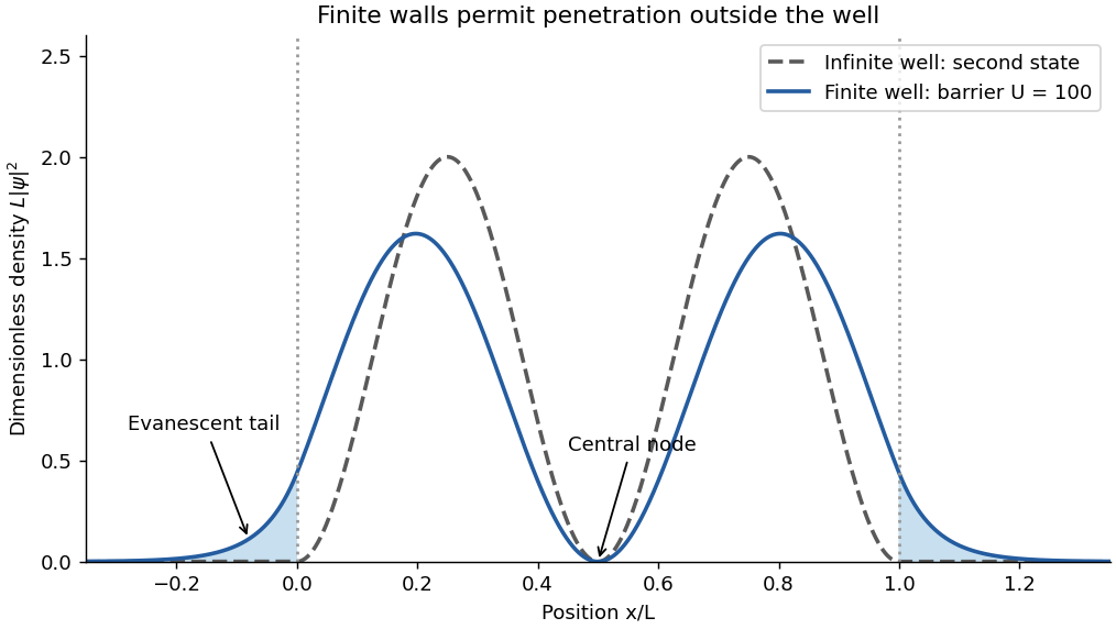
Second-state position densities for an infinite well and an illustrative finite well, including evanescent tails
. Details. Use the dimensionless coordinate :ThereforeThe central interval surrounds a node, which explains why the probability is much smaller than its ten-percent share of the well's length.
The density is symmetric about : . Denote the expectation by . Substitution givesThus . An expectation need not coincide with a high-density position: the centre is a node of this particular state, but the two equally weighted lobes balance about it.
For a symmetric finite well supporting this excited bound state, the wavefunction and its derivative match continuously at each finite potential step. Outside, where , the solution decays exponentially withThe density therefore extends into the classically forbidden region instead of dropping to zero at the walls. Its interior lobes and normalization change, and the energy is lower than for the corresponding infinite-wall state at the same well bottom. Symmetry preserves the central node for the first excited state. The diagram shows an explicitly illustrative barrier height, not an extra numerical value supplied by the question.
In magnetostatics, Ampère's circuital law isIt relates magnetic circulation around a closed curve to the steady current through a spanning surface. It is especially useful when symmetry makes the tangential field constant on a chosen path: an infinite straight wire gives , while an ideal long solenoid gives approximately inside.
The Biot-Savart law gives the field contribution from the actual current geometry:The cross product determines the direction by the right-hand rule. Integrating around a circular loop of radius gives at its centre. A finite wire segment can also be integrated directly, even though it lacks enough symmetry for an Ampère-loop shortcut. The full steady-current circuit includes a return path; a segment calculation specifies that segment's contribution.
Place the wire on the axis, its endpoints at and , and the observation point at . With current along , points out of the page. Its magnitude givesIn the question's angle convention, and . ThereforeThe minus sign in matters because is the exterior obtuse angle.
For a regular hexagon of side , the perpendicular centre-to-side distance is . Each side subtends endpoint angles with and . Its centre field is consequently .
All six contributions have the same normal direction, soThe direction follows the current's right-hand rule. Equal side lengths alone would not fix an arbitrary distorted hexagon's field; the usual regular-coil geometry is used here.
The regular hexagon has area . Choose with its positive normal parallel to the imposed field. The external magnetic flux is , so Faraday's law of induction givesTaking the stated resistance to determine the loop response,A different initial orientation adds a phase. The sign is with respect to the chosen loop orientation and obeys Lenz's law; reversal of that orientation reverses the signed current. This expression neglects self-inductance, as in the resistive-loop model.
The released examiner commentary is not a complete worked solution set. It records an accepted ambiguity in question 8(d); question 7(e) also requires care about its unstated drag model.[ref]
https://www.whatdotheyknow.com/request/natural_science_tripos_physics_e/response/2127325/attach/3/FOI%202022%20639%20Sullivan%20materials.pdf?cookie_passthrough=1#page=61. Examiner commentary for this paper, released PDF pages 61–64
By dimensional analysis, power has dimensions , mass density has dimensions , and angular velocity has dimensions ; radians are dimensionless. ThusMatching the three independent dimensions gives , and , henceWith unchanged mass density, angular velocity and the same performance coefficient (a dimensionless quantity), the pump power affinity law givesThe required power therefore increases by . This uses the stipulated dependence on only these three quantities, with comparable pump geometry and performance; dimensional analysis alone does not guarantee that unrelated pumps have the same performance coefficient.
The relativistic kinetic energy is the total energy minus the rest energy:Here is the Lorentz factor and the speed of light. The binomial series, with , givesFor , the leading term is the classical kinetic energy . The ratio of the fourth-order term to that leading term is . ConsequentlyThe condition concerns one term of the binomial series; it is not the condition that the entire relativistic correction be exactly .
Let be signed displacement along the rails, measured from the centre. The diagram in the original paper shows a guide extending across the centre, so the signed coordinate can pass through zero. Hooke's law gives the radial force . In the rotating reference frame, the radial centrifugal force is . The Coriolis force is perpendicular to the rails and is balanced by their reaction; it has no radial component. Therefore Newton's second law givesEquivalently, the radial component of acceleration in polar coordinates in the inertial frame is . The radial spring oscillator on a rotating guide has simple harmonic motion only when , withThe angular frequency is in and the frequency in . The critical angular speed isStrictly this is an upper bound, not an attained maximum for oscillations: at equality , so a displaced object released from rest stays at its displaced position relative to the rails; above it, the central equilibrium is unstable.
Take the thin lens at , with the object on the left and light rays travelling to the right. The positive object distance is and the focal length is . The thin lens equation givesThe transverse magnification and signed image height areThus the real image is beyond the lens, inverted and high. For the ray tracing, a light ray parallel to the optical axis emerges through the far optical focus; a light ray through the optical centre continues straight in the ideal thin lens model. They intersect at , independently reading off both answers from the diagram.
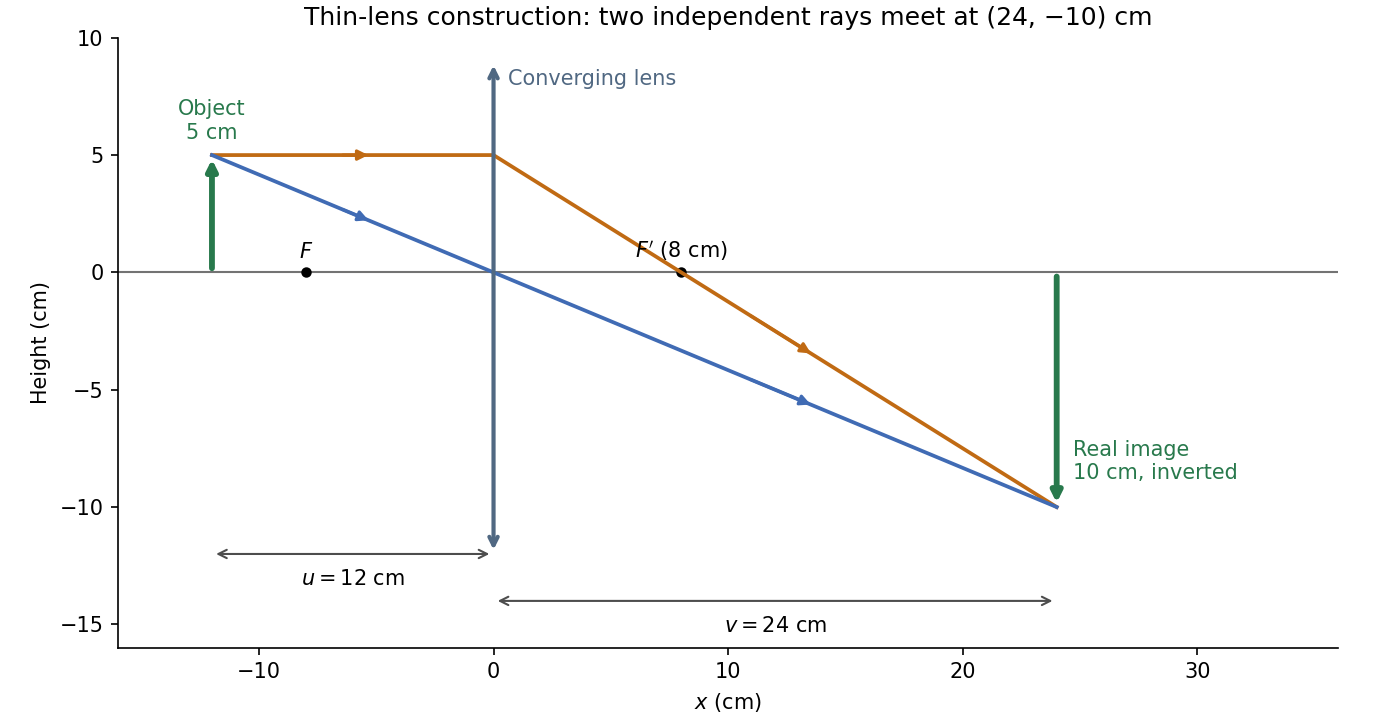


The calculation and diagram use the ideal paraxial approximation implicit in the thin lens equation. The comparatively large object height does not supply enough information to calculate optical aberrations of a real lens.
Write for the side length. In an equilateral triangle, the distance from centre to a vertex is ; it is two thirds of the altitude . By the superposition principle, the electric potential at the centre due to the three fixed electrons isHere is the elementary charge and the vacuum permittivity. The approaching electron has electric charge , so its potential energy, measured relative to infinity, is positive:The fixed sources do not move, and radiation is excluded. Hence conservation of mechanical energy givesUsing , for the electron mass, and givesThis speed is small enough to justify classical kinetic energy. There is an idealization in the word “stops”: along the line normal to the triangle through its centre, this threshold energy makes the electron approach the central equilibrium asymptotically. A smooth, conservative trajectory cannot reach an equilibrium with exactly zero velocity in finite time unless it was already there. The energy threshold, and therefore the requested initial speed, is nevertheless unambiguous.
Choose three mutually perpendicular axes through the same point, and label coordinates . The moments of inertia of any rigid body areSubtracting givesFor a thin planar lamina lying in , the right-hand side vanishes, proving the perpendicular axis theorem:The two in-plane axes and the perpendicular axis must intersect at one point; this need not be the centre of mass. For an extended three-dimensional mass distribution, the equality generally fails. The general moment-of-inertia triangle inequalities arewith equality in the first precisely when all mass lies in the plane perpendicular to its axis, and cyclically for the others. None of these identities requires principal axes.
Let denote the moment of inertia normal to the disc and that about any central diameter. Rotational symmetry makes the two perpendicular diameter values equal. By the perpendicular axis theorem, . The intended angular impulse has magnitude ; delivering that magnitude about a diameter instead gives . ThusThese are principal axes, so angular momentum is parallel to angular velocity in both cases. Equal delivered angular impulse means equal magnitude of the change in angular momentum, not equal rotational kinetic energy; the actual rotational kinetic energy is twice the intended value.
Take along the upper ship's initial velocity, and take from the lower ship to the upper ship at closest approach. The upper and lower ships then have initial velocities and . Their equal masses put each at distance from the centre of mass, soBy momentum conservation, the centre of mass keeps moving with constant velocityIn that frame the ships have opposite velocities of magnitude . Their initial angular momentum about the centre of mass is nonzero even though their trajectories were straight:The tether exerts central internal forces, so conservation of angular momentum givesEach ship follows uniform circular motion of radius around the translating centre of mass, clockwise viewed from . More explicitly, put the initial centre at the origin and defineThe kinetic-energy decomposition about the centre of mass verifies conservation of mechanical energy directly:At closest approach the relative radial velocity is already zero, so connecting the tether requires no dissipative radial impulse. Subsequently its tension is perpendicular to each ship's velocity relative to the centre of mass and does no net work on the pair at fixed .
Each ship needs centripetal acceleration , supplied entirely by the tension. ThusThe result has units of force, .
During quasi-static tether contraction, momentum conservation keeps constant and conservation of angular momentum keeps constant. To leading order in the slow radial motion, the kinetic energy isIts derivative at fixed , not fixed , isTo compute the power supplied by the tension, use the instantaneous unit vector from the lower to the upper ship. Their radial velocities relative to the centre of mass are , and the tension forces are . ConsequentlyThe translational contributions cancel between the two ships and the tangential contributions are zero. The contraction mechanism supplies positive work, increasing the rotational kinetic energy.
The slow-contraction approximation matters: for a prescribed smooth with a taut tether, the exact kinetic energy and tension include radial terms,These still satisfy . Thus the paper's displayed formula is the leading result for slow, smooth contraction, or is exact when the radial kinetic energy is constant; it is not an identity for every possible shrinking schedule.
Articles were limited to the first 100 out of 656 total.
Articles by others on the same topic
There are currently no matching articles.