
Discrete-jump model of Barkhausen noise 2026-10-18
An explicit constructed model separates slow magnetization drift from discrete collective jumps:Here is the Heaviside step function, the Dirac delta function, a smooth drift rate, and the jump times. The ideal discontinuities stand for events shorter than the resolved timescale; actual magnetic domain walls move over finite times. This equation stipulates jump sizes rather than deriving them from atomic spin. With in the preceding geometry, subtracting the smooth background leaves .
Let a stable linear filter have causal impulse response , normalized by , and let be a constant dimensionless voltage gain. The output is a convolution:A simple low-pass filter has , with time constant . Its output pulse has peak proportional to and signed area . Integrating the convolution proves area preservation because ; a wider filter response lowers peaks and lengthens tails. This ideal filter models resolution, rather than claiming the cited instrument had exactly this response.


The nearby positive jumps in the figure have additive negative pulse areas even when their tails overlap. For the first of the pair still has of its initial height when the second arrives. Thresholding can merge those responses into one detected event; limited signal bandwidth also obscures their separation. The total signed area still records the sum if the complete response is integrated, but cannot identify how that sum was partitioned into events. Equal simultaneous jumps are exactly indistinguishable from a single jump of their summed size in this linear measurement. Oppositely signed simultaneous changes can cancel.
Area preservation requires the stated electronics. A zero-DC stage after the low-pass filter has responseConsequently over the complete response: a main pulse is followed by a compensating tail. Integrating only a threshold-selected lobe, clipping the record, or saturating the amplifier breaks the simple pulse-area inference. Recovering a magnetization change from such a readout needs the calibrated frequency response and an appropriate reconstruction. Neither the audible crackle nor the displayed voltage is a direct staircase of magnetization.
Barkhausen pulse area 2026-10-18
Write the magnetic flux linkage of the stationary pickup coil as , in SI units of weber. If every turn links the same magnetic flux , then ; the turn count is dimensionless. With a fixed winding and terminal convention, Faraday's law of induction gives the induced electromotive forceThis is the fundamental theorem of calculus applied to magnetic flux linkage. Its units are , not volts alone. Reversing the leads reverses the sign. In a high-input-electrical resistance voltage measurement the input approximately follows this electromotive force; coil loading and the frequency response of the electronics require separate calibration.
Separate direct drive linkage from material linkage: . Even an empty pickup coil has . In an ideal long, uniformly coupled specimen with negligible demagnetizing field correction and eddy current shielding, a useful material approximation isHere is specimen cross-sectional area, not the larger coil aperture; is vacuum permeability and the axial magnetization sampled by the coil. The units check directly: . Finite geometry and nonuniform magnetization generally require a calibrated coupling in place of . The exact linkage identity survives that failure of the uniform approximation.
As an original illustrative calculation, stipulate , , and rounded . ThenA uniform change over would give a rectangular pulse of ; over it gives with the same area. Thus pulse height mixes change size with change speed. These numbers describe an ideal model, not observed pulses or material constants.
Inductive Barkhausen experiment 2026-10-18
Heinrich Barkhausen's 1919 report used iron, a 300-turn pickup coil, moving magnet, amplified telephone readout and galvanometer. Removing iron corrected drive pickup. [ref]
The Barkhausen effect by Gianfranco Durin and Stefano Zapperi. Appendix A, p. 46: later translation of the 1919 apparatus and blank control
A modern primary experiment by Gianfranco Durin and Stefano Zapperi used annealed iron–silicon strips and amorphous alloys. A 60 cm solenoid swept a triangular magnetic field intensity; a 50-turn pickup coil, wound within 1 mm, sensed the specimen. A preamplifier with a 3–20 kHz low-pass filter preceded sampling. Measurements selected the central hysteresis region dominated by magnetic domain wall motion. Above-background threshold crossings defined event durations; integrating between crossings defined event sizes. These are reported procedures, rather than data generated for the diagrams.[ref]
Scaling exponents for Barkhausen avalanches in polycrystals and amorphous ferromagnets by Gianfranco Durin and Stefano Zapperi. pp. 1–2: apparatus, specimens and threshold integration
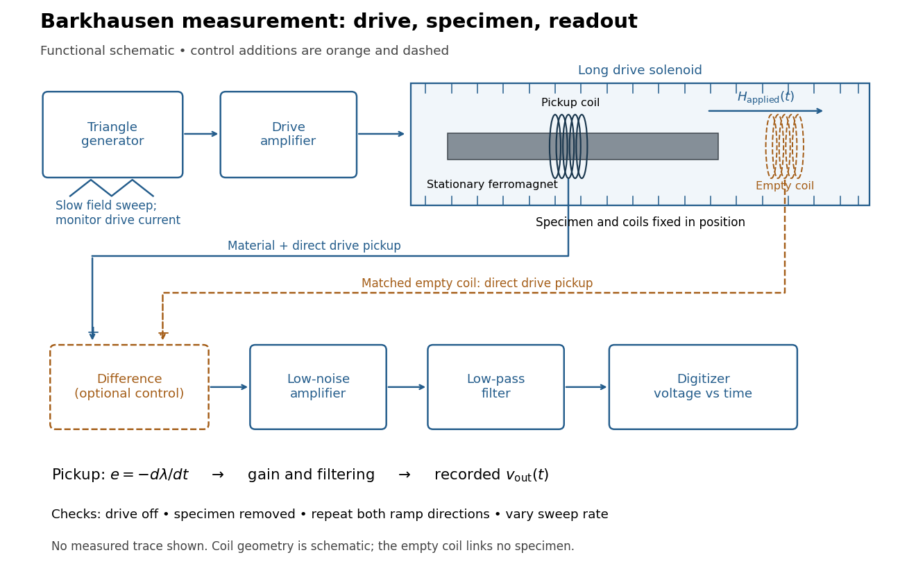
Barkhausen effect: swept magnetic field, stationary specimen and inductive readout
. Original functional schematic of the modern measurement principle. The specimen and pickup coil remain stationary; no torsional suspension or mechanical rotation is needed. The empty matching coil, difference stage and drive monitor show proposed controls, not an assertion that every component was present in the cited 2000 apparatus. The triangle indicates a drive waveform, not measured Barkhausen noise. Details.
For this stationary implementation, secure a thin ferromagnet and its pickup coil inside a longer drive solenoid, keeping their relative positions fixed. Drive the solenoid with a slow triangular electric current, monitor that electric current, and record the amplified, filtered induced electromotive force with a digitizer. A speaker may make suitable frequencies audible, but the voltage record is needed for quantitative analysis. Slow variation of the drive does not require smooth magnetization. A triangular drive supplies an approximately constant applied-field sweep rate along each ramp; it does not guarantee constant instantaneous .
A proposed control sequence makes the inference testable. First record the electronics background with no drive. Repeat the same sweep with the specimen removed, retaining coil geometry: mutual induction from the drive can itself induce a voltage. A matching empty pickup coil wired in opposition can suppress common drive pickup, after checking its matching. Compensation of air flux by an opposed coil is an established method.[ref]
The Barkhausen effect by Gianfranco Durin and Stefano Zapperi. §II.A.1, p. 4: opposed-coil compensation
Then restore the specimen, repeat both sweep directions, reduce sweep rate, and compare the same hysteresis region with fixed amplifier gain, filter and threshold. Monitor drive irregularities and mechanical vibration; either can generate spurious pulses. These controls are recommendations for the schematic, rather than undocumented controls attributed to the modern paper.A genuine material contribution should differ from the blank-coil record and change reproducibly with the magnetic preparation and sweep region. Quieting the drive tests drive-correlated pickup, but a held field need not eliminate all delayed material motion. Reversing the sweep is a consistency check on signed changes, not a demand that individual events retrace. A changing pulse count under a different filter or threshold cannot by itself establish changed microscopic dynamics. The useful inference is intermittent collective magnetization change within the instrument's signal bandwidth, with spatial detail left unresolved.
Direct band gap 2026-10-18
A band gap whose conduction band minimum and valence band maximum occur at the same crystal momentum, allowing an optical transition without a momentum-balancing phonon.
Indirect band gap Created 2026-10-18 Updated 2026-10-20
An indirect band gap separates a valence band maximum and a conduction band minimum at different values of crystal momentum. A near-edge radiative transition then usually needs a phonon or another momentum-transfer process in addition to the photon, whose momentum is small on the Brillouin zone scale. A direct band gap has the extrema at the same crystal momentum and more readily supports efficient band-edge light emission. A material can have direct transitions at higher energy while its smallest gap is indirect.
For with , a nearest-neighbour cubic tight-binding model has zone-centre band effective massIts logarithmic derivative is . The unique minimum occurs at and has value . The explicit in band curvature competes with the exponentially weakening hopping integral. Extrapolation to vanishing atomic separation lies outside the localized-orbital approximation.
Band curvature 2026-10-18
Band curvature is the Hessian matrix of an energy band as a function of wavevector. Dividing it by gives the inverse band effective mass tensor. At a one-dimensional band minimum the curvature is positive, whereas at a maximum it is negative. Near a weak two-wave avoided crossing with reciprocal wavenumber and coupling magnitude , the two edge curvatures are . This is a crystal response coefficient, not a change in the bare electron mass.
In a one-dimensional two-wave nearly-free electron model, set and let the coupling magnitude be . Near the Bragg plane,Expansion at gives , henceThe lower edge has negative electronic curvature, and the upper edge positive curvature. The last expression is a leading weak-potential approximation, not the exact curvature of the two-wave dispersion.
Effective-mass tensor Created 2026-10-18 Updated 2026-10-20
For a semiclassical wave packet in an isolated energy band, and imply . The inverse effective-mass tensor is the Hessian matrix of the dispersion divided by . Along a unit vector , . The Laplacian is its trace: . Thus in isotropic dimensions the scalar mass is , rather than .
Time-dependent neutral-B CP asymmetry 2026-10-18
With CPT symmetry, write the propagating states of neutral meson mixing as , defining the coefficient ratio . Let be their mass splitting and use units .
For rates tagged as and , neglect the decay width difference and take . DefineHere are decay amplitudes. The tagged asymmetry is in this convention.[ref]
For a single weak phase in a charmonium-kaon CP eigenstate with eigenvalue , gives , , withThis connects the CKM unitarity triangle to quantum interference between direct decay and decay after neutral meson mixing.[ref]
Observation of CP violation in the B0 meson system by BABAR Collaboration. PDF p. 4, Eq. (1) and charmonium weak phase
For an independent teaching example choose , and an arbitrary common positive envelope . Then , andBecause , both rates remain nonnegative. At , the asymmetry is ; at , it is . These chosen values illustrate the sign convention and are not experimental estimates. More generally .
If a tag flips independently with probability , exchanging and for that fraction of events gives by direct subtraction. The plotted toy choice reduces the amplitude to of its ideal value; at the tag contains no flavour information. Finite time resolution additionally averages over nearby oscillation phases. Extracting a weak phase consequently requires calibrated readout as well as a CKM matrix prediction.
For boundary data on the sphere , with , define its Legendre polynomial coefficients by . Separation of variables in the Laplace equation gives radial factors and . Regularity at the origin selects the first for the interior Dirichlet problem; decay at infinity selects the second for the exterior problem. Matching each boundary coefficient gives the displayed series. For continuous boundary data the resulting harmonic functions attain those data, with convergence interpreted through their harmonic extension rather than requiring uniform convergence of the unweighted boundary series. The maximum principle for harmonic functions proves uniqueness in the bounded interior and decaying exterior classes.
Arcsine distribution on a bounded interval 2026-10-18
Specify whether two parameters mean endpoints or location and width. With endpoints , define for a standard arcsine distribution variable . ThenThis is a location-scale family with location and width . Its mean is and its variance is . A convention using parameters for location and width instead has right endpoint , so it must not be read as having endpoints .[ref]
The Arcsine Distribution. Random: Probability, Mathematical Statistics, Stochastic Processes by Kyle Siegrist; The General Arcsine Distribution, Definition, Distribution Functions and Moments: location-plus-width convention and alternative endpoint parametrization
For example, a chosen interval gives mean and variance , while its density still concentrates toward both endpoints. It is a bounded probability distribution; its endpoint singularities do not make its support infinite.
Arcsine quantiles and moments 2026-10-18
Inverting gives the quantile functionConsequently, inverse transform sampling uses with uniform on . The quartiles are , and .[ref]
The Arcsine Distribution. Random: Probability, Mathematical Statistics, Stochastic Processes by Kyle Siegrist; The Standard Arcsine Distribution, Distribution Functions and Related Distributions: quantiles, quartiles and random quantile construction
The first and third quartiles are about and , so the central half of the probability spans about of the unit interval. Under a uniform distribution, its width would be .
The symmetric probability distribution gives . The angle representation gives a short calculation of the second moment:Use to evaluate the integral. A uniform distribution on has variance ; the larger variance quantifies the greater spread toward the ends.
More generally, for a nonnegative integer , the beta function yieldsFor this is one; for it reproduces the values above. The central binomial coefficient thus appears in an exact moment calculation for a continuous probability distribution.
An unbounded probability density function does not imply an atom. HereThe last equivalence follows from . The endpoint interval has much more probability than the same interval under a uniform distribution, whose value is , but its probability still tends to zero. This is an integrable singularity.
For example, the first 1% of the unit interval contains about of the probability; the last 1% contains the same amount because the arcsine distribution is a symmetric probability distribution. Each exact endpoint still has zero probability. Density and interval probability answer different questions.
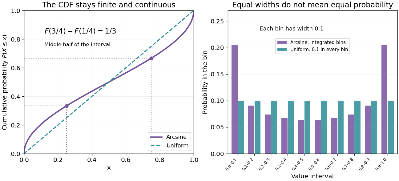
Endpoint density diverges, but every finite bin has finite probability
. Original exact curves and bin probabilities. Left: the arcsine cumulative distribution function compared with the uniform one. Right: ten equal-width bins have probabilities , not heights sampled from the divergent density. Their total is one. Details.
A numerical integration routine must respect these endpoint integrable singularities. The substitution givesIt turns a difficult-looking density integral into a constant measure in angle. Integrating finite bins is also a faithful way to draw the distribution near its endpoints; sampling to make a bar height is not.
Arcsine distribution from a uniform angle 2026-10-18
Choose with uniform distribution on and set . Since the sine is increasing on this interval,Differentiation gives , and , prove normalization. This also evaluates the density's improper integral without treating its divergent endpoint values as infinite probability.
For the circle construction, instead choose with uniform distribution on and put . Each has two preimages in one revolution. The change of variables formula adds both contributions:The affine change of variables gives the standard arcsine distribution. A single monotone-branch calculation without the second preimage would give only half the total probability.
The same geometry explains the ideal harmonic oscillator , with amplitude and angular frequency . Choose uniformly in any complete period of duration . Its oscillation phase modulo is uniform, and has densityNear a turning point, is small, so a fixed position interval takes more time to cross. For the chosen amplitude , exactly one third of the period is spent in , and two thirds outside that central interval. These are calculations for an ideal sinusoid, rather than measured oscillator data.
The sampling assumption matters. Taking one observation every full period returns the same position each time. It does not produce this probability distribution. Uniformly random observation times and a fixed regularly spaced sampling scheme are different models; aliasing can conceal the motion altogether.
Paul Lévy used a related geometric construction in his work on stochastic processes: project a uniformly chosen point on a circle onto its diameter to divide a segment. The projection description appears explicitly in §5 of his paper, following its arcsine density calculation.[ref]
For a real antisymmetric matrix, transpose gives , so this trace vanishes. Every complete pairwise tensor contraction of copies of , using the Euclidean Kronecker delta, splits into closed index cycles. Each cycle is a trace of a power of , up to a sign from index order. An odd total number of copies forces an odd-length cycle, so the whole contraction vanishes. This assertion concerns pairwise index contraction with the metric; inserting additional tensors would be a different claim.
Lagrange multiplier for antisymmetry 2026-10-18
To vary an antisymmetric tensor without treating its entries as independent physical variables, temporarily allow an unrestricted array and add to the Lagrangian density, with symmetric Lagrange multiplier . Variation of enforces antisymmetry. The antisymmetric part of the unrestricted equation eliminates and gives the physical Euler-Lagrange field equation. Equivalently, vary only the six independent entries in four spacetime dimensions. Quadratic contractions must be differentiated before applying antisymmetry, or their factors and signs can be lost.
Antiproton Created 2026-10-18 Updated 2026-10-25
The antiproton is the antiparticle of the proton: it has the same rest mass and spin , with opposite electric charge and baryon number. A negative electric charge alone cannot identify an antiproton, because a negative pion also bends in that direction in a magnetic field. Combining magnetic rigidity with velocity determines a rest mass; agreement with the proton rest mass then makes the identification much more discriminating.
The mode expansion of a Dirac field explains how independent particle and antiparticle excitations enter a relativistic field description. It supplies a theoretical language for the antiproton, while the Chamberlain-Segrè antiproton identification supplies an experimental test. The proton is a composite baryon, so a free Dirac field is not a complete account of its internal dynamics or of antiproton production in a target.
Snoek effect 2026-10-18
The Snoek effect is anelasticity caused by stress-induced redistribution of mobile interstitial defects among differently oriented sites in a crystal. An applied stress favors orientations whose local distortion best accommodates it. At low frequency the atoms can track that bias and provide additional relaxed compliance; at high frequency their populations are nearly frozen. Dissipation is largest between these regimes. For a weak single relaxation, the loss tangent has the approximate shape , with for thermally activated hopping. The peak is near . This describes a standard mechanism for interstitial impurities in body-centred cubic metals, not every damping mechanism in every alloy. [ref]
https://www.jstage.jst.go.jp/article/isijinternational1989/37/6/37_6_610/_pdf. ISIJ International 37 (1997), 610: stress-induced interstitial diffusion, Eq. (2) for the Debye-shaped damping peak and its activated relaxation time
Discrete gauge cancellation in two-path interference Created 2026-10-18 Updated 2026-10-20
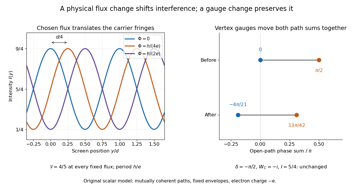
A four-vertex model proves the essential gauge invariance without solving an electron scattering problem. Use two directed paths and . Assign an edge phase and a complex unit link to each directed edge, with . These links represent discretized magnetic line integrals multiplied by . Under a gauge transformation with arbitrary vertex phases ,Both path products acquire the same factor . Their gauge-invariant ratio is the closed-loop holonomyEvery intermediate vertex phase cancels. For any fixed nonnegative real amplitudes , the interference quantity is unchanged too. A gauge-dependent open-path phase consequently cannot be interpreted as an observable by itself.
For an exact example, measure phases in units of and order edges as . Choose edge phases and vertex phases . The transformed edge phases areThe upper and lower sums become and ; their difference remains . With amplitudes , , the intensity remains . Sweeping one physical loop phase through instead produces extrema and , agreeing with the interferometric visibility example above.

There are unlisted articles, also show them or only show them.