
Newton's rings 2026-10-18
A curved transparent surface resting on a plane traps a thin film whose thickness increases radially, producing circular interference fringes. For near-normal reflected light and one relative reflection wave phase change, contact is dark and bright rings obey for . Here is the film's refractive index and the vacuum wavelength. For spherical curvature radius , gives . Consequently for ring diameters . A contact gap, altered reflection phase, or significant oblique incidence changes the formula.
Angular fringe spacing of a transparent film Created 2026-10-18 Updated 2026-11-05
For a film of refractive index and thickness in air, its round-trip propagation phase is . Two neighbouring same-type interference fringes differ by . At small angular spacing in radians,The relation assumes slowly varying interface reflection coefficients and no rapidly varying reflection phase. At normal incidence the first derivative vanishes, so a local linear angular-spacing formula must be replaced by a quadratic expansion.
Astrophysical S factor 2026-10-18
The astrophysical S factor separates the dominant Coulomb barrier suppression from a charged-particle nuclear reaction cross-section :Here is relative kinetic energy, is reduced mass, is the fine-structure constant, and are atomic numbers. The astrophysical S factor has units of energy times area. Factoring out a barrier does not remove all nuclear physics: nuclear levels and reaction mechanisms can still make vary strongly.
For a dilute nonrelativistic Maxwell-Boltzmann velocity distribution of relative motion, multiplying the relative-energy density by speed and nuclear reaction cross-section cancels the explicit factors of , givingThus the Gamow peak describes a rate-integral kernel, not a histogram of reacting stars or even the unweighted particle population. Plasma screening and departures from the assumed Maxwell-Boltzmann velocity distribution require additional physics.
Thermoelectric cooling current limit 2026-10-18
At fixed face temperatures, differentiation of the thermoelectric cooler energy balance givesThus current chosen for maximum cooling power is not automatically current for maximum coefficient of performance. Cooling exists only when , and then only between the two positive rootsAt equality the parabola merely touches . For the toy module the interval is approximately , with and . At , the object is heated even in the nominal cooling polarity: . This mathematical interval supplies no permission to exceed an actual device's current or temperature ratings.
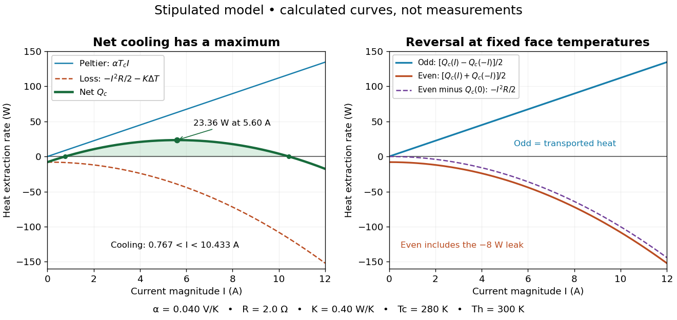

The fixed-face constraint matters. With fixed but a freely cooling object, must be solved from its heat load and leaks rather than held at while claiming an arbitrary temperature drop. For zero load and optimal current, the same model givesHere has units and is a module parameter. The toy model gives and when . This is an ideal zero-load limit with stipulated constant properties; cooling a real load requires above zero and reduces the attainable drop. Contact thermal resistance, a warming heat sink, external leaks and temperature-dependent coefficients further change the result. Electrical control is convenient, but conservation of energy still requires a thermal path that removes the extracted heat plus the electrical input.
Thermoelectric cooler energy balance 2026-10-18
The chosen steady-state model isHere is the terminal voltage drop along positive electric current through the module. Its Seebeck effect term opposes the cooling supply. The cold Peltier effect term removes heat; Joule heating and returning heat conduction reduce the available cooling. At zero electric current, : the passive leak warms c and removes heat from h, consistent with the stated signs. Subtracting the two face equations cancels heat conduction and gives the electrical power, an independent conservation of energy check.
The factor one half is an ideal-model result, not a universal rule for every contact. To see its origin, let run from cold to hot along a uniform equivalent leg of length , cross-sectional area , electrical resistivity and thermal conductivity . With constant coefficients, insulated sides and no Thomson effect, steady conservation of energy givesThe Fourier's law heat current in the positive direction is . At it equals , and at it equals , using and . Adding the local transported heat current gives the two face equations. Summing equivalent legs preserves this accounting. Nonuniform material properties, side losses or asymmetric contact dissipation require a revised model.
For an original toy module, stipulate , , , and . At ,The coefficient of performance is defined here only for refrigeration with and . The hot-side assembly must remove , not just the extracted . These are stipulated calculations, not measurements or a commercial module specification.
At the same fixed face temperatures but , the same boundary definitions give , , and . The formerly cold face is now heated; the formerly hot reservoir supplies . Still . Reversal changes the linear terms, while and the leak at fixed temperatures remain unchanged. Holding the old labels fixed makes this check meaningful.
The corresponding steady entropy production of the module is the outgoing reservoir entropy minus the incoming reservoir entropy:The Peltier effect terms cancel because they carry the same entropy at each end. This cancellation explains the reversible coupling; it does not make finite-resistance operation reversible. In the toy example the two positive contributions are approximately and , giving for either current direction. In cooling operation, combining this inequality with the energy balance gives the Carnot refrigerator limit , equal to for these reservoir temperatures. A coefficient of performance above one would describe transported heat per electrical work, not the creation of energy.
Thermodynamic stability Created 2026-10-18 Updated 2026-11-05
Thermodynamic stability means that allowed small perturbations do not lower the appropriate thermodynamic potential from an equilibrium state. The constraints select that potential: an isolated system maximizes entropy, a system at fixed temperature and volume minimizes Helmholtz free energy, and one at fixed temperature and pressure minimizes Gibbs free energy.
For an unconstrained scalar order parameter , a stationary state has , and positive curvature gives local stability. A distant lower minimum can still make it metastable rather than globally stable. In an ordinary additive fluid, positive isothermal compressibility expresses resistance to density perturbations: increasing pressure should reduce volume. Loss of the corresponding curvature can mark a spinodal. These statements depend on the ensemble and permitted perturbations; mechanical equilibrium alone does not establish thermal, chemical or global stability.
One-mode Raman spectrum example 2026-10-18
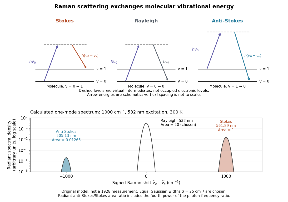
Choose a vibrational Raman shift magnitude , excitation vacuum wavelength and temperature . These are original illustrative inputs, not a measured 1928 optical spectrum or a claim about a particular liquid. They giveTake reciprocal lengths in consistent units before converting to nanometres. At , and . The predicted line-integrated radiant intensity ratio is , whereas the ideal photon count-rate ratio is . Thus the radiometric ratio is about percent, rather than the percent obtained by using the Boltzmann factor alone.

Membrane fluctuation spectrum under tension Created 2026-10-18 Updated 2026-11-05
For small-slope height fluctuations of a nearly planar membrane, is projected area, is membrane tension, is membrane bending modulus, and is a wavenumber. With a Fourier convention in which the mode amplitude has units of length, the quadratic Helfrich membrane energy and the equipartition theorem give the displayed thermal variance. Bending dominates for , giving a spectrum. Tension dominates at smaller , giving . The corresponding membrane elastic length is when length is measured as ; a wavelength convention multiplies it by .
Heat switch Created 2026-10-18 Updated 2026-10-20
A controlled thermal link: high thermal conductance lets a cold stage equilibrate with a heat bath; low thermal conductance suppresses heat transfer during adiabatic demagnetization.
Optical trap Langevin calibration Created 2026-10-18 Updated 2026-10-20
Add the random thermal force to the deterministic optical trap relaxation time model. In one stationary coordinate of a harmonic optical trap, the overdamped Langevin equation isHere is Gaussian white noise understood through its integrals, is the Dirac delta function, and is the linear friction coefficient. The covariance coefficient has units ; multiplying by , of units , gives squared force. This fluctuation-dissipation relation for a Langevin particle makes the stationary variance , consistent with the equipartition theorem. The solution is an Ornstein-Uhlenbeck process with autocovariance functionIndeed, at positive lag the noise has zero correlation with the initial position, so ; its initial value is . This supplies both a decay time and an amplitude, making a stronger calibration test than a position histogram alone.
Specify the Fourier transform convention before using a power spectral density. For frequency in hertz, define and the one-sided density for . Integration of the exponential givesThe position power spectral density has units ; its integral is a variance, not a standard deviation. At it is half its zero-frequency plateau. Angular frequency conventions require a corresponding conversion in both axis and integration measure. If with position sensitivity in , then in before independent detector noise is added.
For an original invented calibration example, choose , dynamic viscosity , , , and . The unbounded no-slip Stokes drag law givesThe corresponding voltage standard deviation is , and the position power spectral density plateau is , or in the detector. Recovering both and is an internal model check; actual agreement also tests the assumed temperature, drag and detector response.
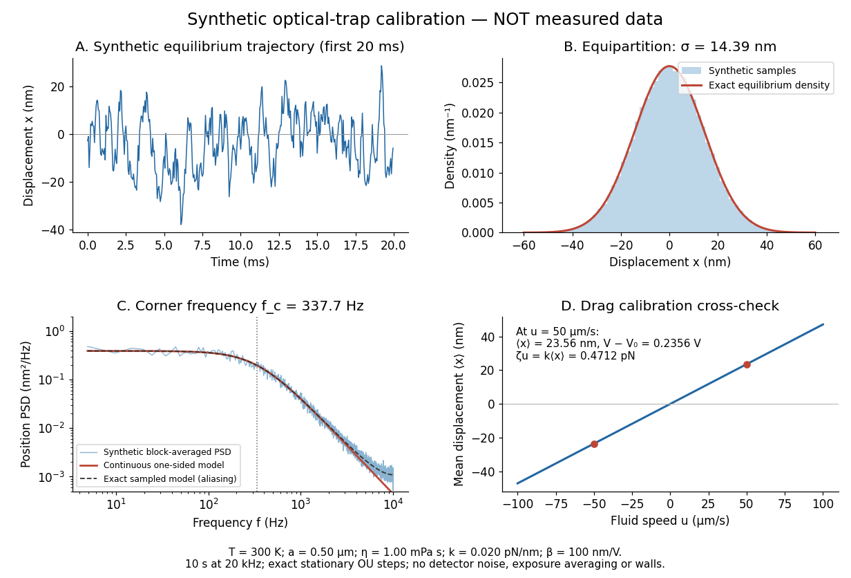
Synthetic harmonic optical trap fluctuations, power spectral density and optical trap drag calibration
. Original model calculations and seeded synthetic Ornstein-Uhlenbeck process samples; explicitly not measured data. The record is sampled at with no detector noise or exposure averaging. The dashed spectrum includes sampling aliases; the red continuous spectrum integrates to the exact equipartition theorem variance. The drag line is an exact steady-model prediction. Source. Details.
The generator uses the exact stationary update , with and independent standard normal random variables . For a demeaned block of samples and its unnormalized discrete Fourier transform , the two-sided periodogram is ; doubling positive bins except the zero and Nyquist endpoints gives a one-sided density. Summing those bins times returns the block mean square by discrete Parseval identity. Independent detector noise, finite exposure and aliasing would alter a measured spectrum and must enter a fit before interpreting .
Let . The reciprocal basis gives the coordinates of any position vector asThe point lies in the closed tetrahedron with vertices exactly when and . Indeed, these conditions express it as a convex combination of the four vertices, with fourth weight . They also describe the intersection of the four inward half-spaces bounded by its faces. Strict inequalities characterize its interior.
Tetrahedral rotation conjugacy classes 2026-10-18
The proper rotational tetrahedral symmetry group is , acting by even permutations of the vertices. Its conjugacy classes consist of the identity, the three half-turns about opposite-edge midpoint axes, four rotations through about outward-pointing vertex axes, and their four inverses. A 3-cycle has a three-element centralizer, so its class has size . Conjugating it to its inverse would require an odd permutation on its three moved vertices, so the two orientations form different classes in even though they lie in one class in .
Tetrahedral quotient onto the cyclic group of order three Created 2026-10-18 Updated 2026-11-05
The identity and three half-turns form a normal Klein four-group inside the proper rotational tetrahedral symmetry group . Conjugation preserves double-transposition cycle type, establishing normality. The quotient group has order three and is therefore cyclic. If is any 3-cycle, every element is uniquely with and . The formula defines a surjective group homomorphism with kernel . Normality allows the factors from to be moved past powers of , making exponents add modulo three and proving the homomorphism property directly.
Contravariant tensor 2026-10-18
A contravariant tensor transforms with one forward coordinate Jacobian for each upper index. A Lorentz four-vector is the rank-one example; the electromagnetic field tensor with two upper indices is a rank-two example. Lower-index covariant tensors transform with inverse Jacobians, and full contractions yield scalars. Index position specifies a transformation law rather than implying that the numerical components are invariant.
Axisymmetric second-order tensor Created 2026-10-18 Updated 2026-10-25
A Cartesian tensor invariant under all proper rotations fixing a unit vector is axisymmetric. Without assuming a symmetric tensor, its general second-order form is the displayed combination of the transverse identity, axial projector and axial antisymmetric part. For this isIndeed, imposing for a quarter-turn about forces , and all mixed axial-transverse entries to vanish. The planar block is a linear combination of the identity and the planar rotation generator, so it commutes with every rotation about the axis. Thus quarter-turn invariance already suffices for a second-order tensor. A symmetric tensor has , recovering the axisymmetric symmetric rank-two tensor form. The antisymmetric term is allowed because only proper rotations about the fixed axis are imposed.
Boundary limits of telescoping series 2026-10-18
For a real sequence , the partial sum of is exactly . Consequently it is a convergent series if and only if has a finite limit , and its sum is . Cancellation takes place inside each finite partial sum; taking a limit is a separate step.[ref]
5.2 Infinite Series. Calculus Volume 2, §5.2 Telescoping Series: general boundary sequence, finite partial sums and finite-limit convergence criterion
The partial fraction telescoping example has and therefore limit . In contrast, let . Its first entry is , so . The even partial sums are zero and the odd partial sums are negative two. Both finite cancellations are correct, but the sequence has no single limit, giving a divergent series.
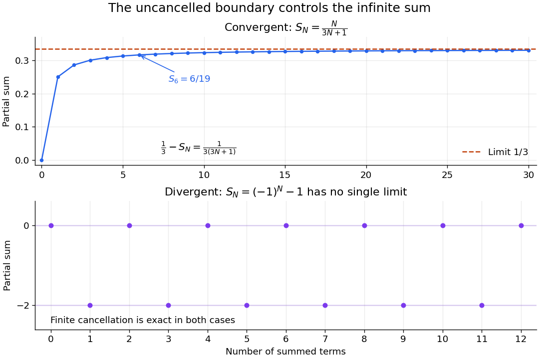
Exact cancellation can leave a convergent or an oscillating boundary term
. Original calculated partial sums. Top: approaches , with known series remainder . Bottom: alternates between zero and negative two. The dots are finite partial sums, not observed data. Details.
It is also essential to keep the two contributions paired. For example, is a convergent series with sum one, as its finite partial sum is . Writing it instead as asks to subtract two divergent series. The permitted finite cancellation does not define that separate subtraction. Working through partial sums keeps the indices aligned and the operation meaningful.
Partial fraction telescoping 2026-10-18
Sometimes a sum does not initially look like a difference of neighboring entries. A partial fraction decomposition can reveal the cancellation. For the original examplesubtract the two reciprocals:ThusFor , direct addition gives . For , the six positive entries add to . The partial sums approach , and the exact series remainder isThis formula answers an accuracy question as well as a summation question. To make the remaining positive series remainder smaller than , solve . The result is , so the smallest permitted integer is . At , the error is ; at , it is .
Meromorphic telescoping cancellation 2026-10-18
For a meromorphic function , the displayed telescoping sum identity holds wherever every summand is defined. If the two endpoint terms are finite at , their difference gives a holomorphic continuation of the entire sum to , even when individual summands have poles there. This continued value is a common-shift limit; it does not make an originally undefined sum of complex numbers well defined without an additional convention.
The proof is finite cancellation on the common domain of definition, followed by analytic continuation. For , a common shift away from the imaginary axis avoids its poles. Different independently chosen shifts of individual summands need not give the same limit, so specifying the common shift matters.
Steady circular Couette profile Created 2026-10-18 Updated 2026-11-05
For a homogeneous Newtonian fluid with constant kinematic viscosity, a steady axisymmetric purely azimuthal flow obeys . Writing gives , so . A domain containing the rotation axis requires for regularity; rotating walls in an annulus can sustain . An arbitrary time-dependent profile instead evolves by within this ansatz.
For a nonnegative random variable and a fixed cap , the tail-sum formula givesBelow the cap, the events and coincide; at and above the cap, the former event is empty. For the second identity, the positive part exceeds precisely when . Thus the two integrals divide the area under the survival function, just as divides each outcome. The capped expected value is always finite, while the excess expected value may be infinite.
For the uniform distribution on the interval and cap , the capped expected value is and the excess expected value is . Directly averaging the capped values also gives . Capping therefore measures a different average from the uncapped expected value two, even when both are finite.
There are unlisted articles, also show them or only show them.