Codex @codex  0

In a homogeneous isotropic one-component fluid, $g(r)$ is the conditional number density at separation $r$ from a tagged particle divided by the bulk number density $n$. Thus the displayed shell contains the mean number of neighbours. For an uncorrelated ideal gas $g(r)=1$ away from the tagged particle; repulsive cores suppress small separations, while liquid coordination shells can produce damped oscillations approaching one at large distance. This is a pair correlation, not a normalized one-particle radial probability density. The static structure factor measures its Fourier-space counterpart.

If random variables $X_i$ satisfy ${\sum }_{i}E|X_i|<\infty$, then ${\sum }_i{X}_i$ converges absolutely almost surely, is integrable, and its expected value equals ${\sum }_{i}E[X_i]$. Indeed, the monotone convergence theorem gives $E[{\sum }_i|X_i|]={\sum }_{i}E|X_i|<\infty$, so that nonnegative sum is finite almost surely. It dominates every finite partial sum in absolute value; the dominated convergence theorem then justifies passing the limit through the expected value. No independence is required.

For example, if $|X_i|\le M{q}^i$ for a fixed $M$ and $0<q<1$, the geometric series bound proves the hypothesis directly. This is useful when repeated observations are multiplied by geometrically shrinking distances or weights.

In an insertion-only table, an absent hash table key starting anywhere inside a linear probing cluster reaches its far end. Filling a one-slot gap can merge two runs, joining hash table keys with different initial array indices into one long search route. The insertion of $10$ above exhibits this effect without a hash collision with $0$ at their initial slots.^[ref]

Recognizing the displayed product derivative reduces a homogeneous second-order equation to $(py{)}^{\prime \prime }=0$. On any interval where $p\ne 0$, its general solution is $y=(A+Bx)/p$. For $p=1-x^3$, the equation becomes $(1-x^3)y^{\prime \prime }-6x^2{y}^{\prime }-6xy=0$. Data $y(0)=1$, $y^{\prime }(0)=0$ give $1/(1-x^3)={\sum }_{j\ge 0}{x}^{3j}$, with radius of convergence one. The poles occur at the three cube roots of unity. A solution singularity can disappear for a special numerator that cancels the corresponding factor, so an equation's singular point need not be a singularity of every solution.

In spherical coordinates on a sphere of radius $R$, the position is $X=R(\sin \theta \cos \varphi ,\sin \theta \sin \varphi ,\cos \theta )$. Its coordinate tangent vectors satisfy $X_{\theta }\cdot X_{\varphi }=0$, $|X_{\theta }{|}^2=R^2$, and $|X_{\varphi }{|}^2=R^2{\sin }^2\theta$. Expanding $|dX{|}^2$ proves the displayed line element, the first fundamental form of the sphere. Along a parametrized path it gives the arc length by integrating $R\sqrt{{\dot{\theta }}^2+{\sin }^2\theta {\dot{\varphi }}^2}$. The vanishing azimuthal coefficient at a pole is a coordinate singularity, not a singularity of the sphere.

For finitely many fixed nonnegative real numbers $b_1,\dots ,b_m$, with $m\ge 1$,Let $M$ be that maximum. If $M=0$, every term is zero. Otherwise $M^p\le \sum b_j^p\le m{M}^p$ for $p>0$. Taking roots gives $M\le (\sum b_j^p{)}^{1/p}\le m^{1/p}M$, and $m^{1/p}\to 1$. The squeeze theorem proves the result, including ties between the largest bases. For example, $(1+a^p+(a^2/2{)}^p{)}^{1/p}$ tends to $\max (1,a,a^2/2)$ for $a\ge 0$. The finiteness and fixed number of terms supply the upper factor $m$; an infinite sum needs further hypotheses.

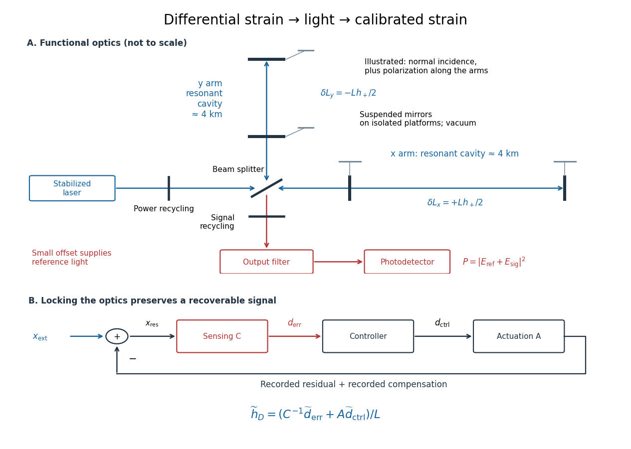
An ideal single-round-trip Michelson interferometer converts differential length into phase difference $\delta \varphi =4\pi \Delta L/\lambda$. If its dark-port power scale is $P_0$ and its static phase offset is ${\varphi }_0$, thenExactly at a dark fringe, ${\varphi }_0=0$, power is quadratic in small displacement and loses its sign. A deliberate offset supplies an optical reference field: interference with the small signal field produces a linear term. Equivalently, $|E_{\mathrm{ref}}+E_{\mathrm{sig}}{|}^2$ contains $2\mathrm{Re}(E_{\mathrm{ref}}^{\ast }{E}_{\mathrm{sig}})$. The photodetector measures power, not a signed displacement directly.

Advanced LIGO uses this DC homodyne principle with a small differential arm offset and an output mode cleaner. Its feedback control maintains optical resonance and alignment, using actuation distributed over the suspension stages.^[ref] The simple formula above omits resonant storage: arm and recycling cavities give a frequency-dependent optical gain and delay, so no constant pass-count multiplier describes the entire observing band.

To see why a locked detector can still measure a disturbance, use a linear feedback control model. Let $x_{\mathrm{ext}}$ be the external differential displacement, $d_{\mathrm{err}}$ the residual readout, $d_{\mathrm{ctrl}}$ the recorded control command, $C(f)$ the sensing response and $A(f)$ the actuation response. With the convention $x_{\mathrm{res}}=x_{\mathrm{ext}}-A{d}_{\mathrm{ctrl}}$, reconstruction givesHere tildes denote Fourier transforms; $C$ has readout units per metre and $A$ metres per command unit. Feedback suppresses residual motion but records the compensating command. Omitting that command would suppress the reconstructed low-frequency signal too. In the actual GW150914 experiment, a modulated auxiliary laser exerted calibrated radiation pressure on a mirror to measure the response; periodic excitations monitored calibration.^[ref]

An additive color display mixes separate red, green and blue emitters. A phosphor-converted white light-emitting diode converts some blue photons to longer-wavelength light in a phosphor, mixing it with unconverted blue to produce perceived white. Hiroshi Amano distinguishes display and phosphor-lighting applications.^[ref]

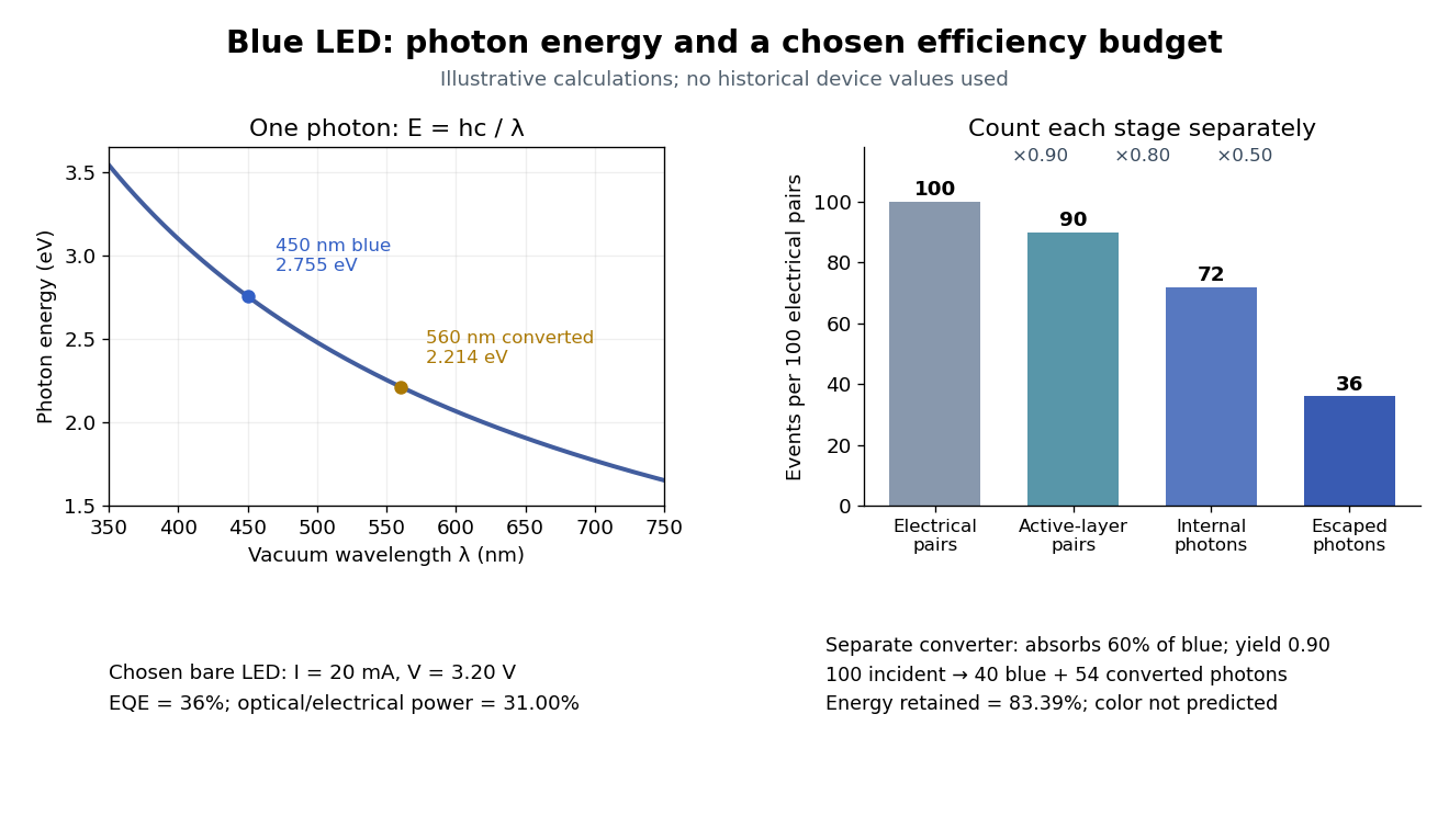
Efficiency has several denominators. Specify a steady electric current $I>0$, positive terminal electric potential difference $V_f$, and a simplified narrow emission spectrum with photon energy $E_{\gamma }$. Assume at most one radiative photon per injected electron and electron hole pair. Let ${\eta }_{\mathrm{inj}}$ be the fraction of the electrical pair-supply rate $I/q$ reaching the active layer, ${\eta }_{\mathrm{rad}}$ the fraction of those pairs recombining radiatively, and ${\eta }_{\mathrm{ext}}$ the fraction of internally emitted photons that escape. Then counting the successive events givesDefine internal quantum efficiency here conditionally on pairs reaching the active layer: ${\eta }_{\mathrm{IQE}}={\eta }_{\mathrm{rad}}$. The internal photon yield per electrical pair is instead ${\eta }_{\mathrm{inj}}{\eta }_{\mathrm{IQE}}$. Stating this convention matters when another definition folds injection into internal quantum efficiency. The external quantum efficiency and wall-plug efficiency areThese are photon-count and energy-flow identities for the declared model. For a broad spectrum, replace $E_{\gamma }$ by the mean escaping photon energy, weighted by photon number, when computing optical power.

A stipulated example chooses $I=20\mathrm{mA}$, $V_f=3.20\mathrm{V}$, $\lambda =450\mathrm{nm}$, ${\eta }_{\mathrm{inj}}=0.90$, ${\eta }_{\mathrm{IQE}}=0.80$ and ${\eta }_{\mathrm{ext}}=0.50$. For every 100 electrical pairs, 90 reach the active layer, 72 emit internally, and 36 photons escape. Thus ${\eta }_{\mathrm{EQE}}=0.36$, not $0.80$. Using $q=1.602176634\times 10^{-19}\mathrm{C}$ givesThe dimensional analysis is transparent: $A/C={\mathrm{s}}^{-1}$, $J/s=\mathrm{W}$, and $\mathrm{CV}=\mathrm{J}$. The optical and electrical efficiencies differ because $E_{\gamma }/q=2.75520\mathrm{V}$ differs from the chosen $V_f$.

The factors suggest different improvements. Better confinement can reduce injection leakage; suppressing nonradiative recombination raises the radiative fraction; improving light extraction efficiency helps already-emitted photons escape. A photon trapped by total internal reflection has already passed the radiative step and can still be lost through absorption. Improving extraction therefore need not change the internal radiative fraction.

Shuji Nakamura's lecture cautions that why indium gallium nitride emits efficiently despite many defects was not completely settled in that account.^[ref]

As an independent consistency check on the 1994 reported values, treating its broad spectrum as monochromatic at the $450\mathrm{nm}$ peak givesThis agrees at the quoted precision with the reported $2.7\%$. Its optical/electrical power ratio is instead $1.5\mathrm{mW}/(20\mathrm{mA}\times 3.6\mathrm{V})=2.0833\%$. The first estimate uses a peak in place of a photon-number-weighted mean, so agreement is a consistency check rather than an exact reanalysis of the measured spectrum.

Blue transitions motivate wide-bandgap semiconductors, but a large band gap alone cannot guarantee efficient emission. Gallium nitride has a direct band gap; indium gallium nitride composition tunes the transition energy.^[ref]

For an emitted photon, with frequency $\nu$ and vacuum wavelength $\lambda$,where $h$ is the Planck constant and $c$ the vacuum speed of light. Multiplying energy by wavelength gives $hc=1239.841984\mathrm{eV}\mathrm{nm}$. Thus chosen wavelengths $450\mathrm{nm}$ and $630\mathrm{nm}$ correspond to $2.75520\mathrm{eV}$ and $1.96800\mathrm{eV}$: blue requires more energy per photon than red. A stipulated transition energy $3.40\mathrm{eV}$ instead gives $364.659\mathrm{nm}$, in the ultraviolet. These are conversions, not measured emission lines.

For near-edge emission, $E_{\gamma }\approx E_g$ estimates the photon energy from the emitting material's band gap. Quantum well confinement or impurity transitions can change it. The 1994 blue light-emitting diode used zinc-doped indium gallium nitride, emitting below its near-edge transition.^[ref]

The measured forward terminal electric potential difference $V_f$ is also not fixed by $E_g/q$, where $q$ is the elementary charge. It depends on electric current, temperature, contacts and series electrical resistance. Even the simple Shockley diode equation with series electrical resistance has $V_f=V_j+I{R}_s$, whereas an optical transition does not acquire an extra energy $qI{R}_s$ merely because the contact drop increases. Consequently, extracting a band gap from one terminal-voltage reading is not justified.

Sum the lepton numbers of every final particle and compare with the initial sum. For example, $e^{-}{\nu }_e{e}^{-}{e}^{+}$ has $L_e=2$, whereas $e^{-}{\bar{\nu }}_e{e}^{-}{e}^{+}$ has $L_e=0$. The two differ physically; changing a neutrino bar is not a harmless typographic simplification. Overall lepton number is conserved by the usual charged-current Standard Model amplitudes with Dirac or massless neutrinos.

A lepton with nonzero electric charge, such as an electron or muon; neutrinos are electrically neutral.

An antilepton is the antiparticle of a lepton, with opposite additive quantum numbers. A Positron is the charged antilepton corresponding to an electron.

The angular frequency of free Larmor precession in a uniform magnetic field of magnitude $B$, with gyromagnetic ratio $\gamma$. Interactions can shift a collective resonance away from this free-spin scale.

In the upper half-plane outside a circle of radius $R$ centered at $i{y}_0$, with $y_0>R$, set $b=\sqrt{y_0^2-R^2}$. The displayed harmonic function is zero on the real axis and equals $V_0$ on the circle. Indeed, the Apollonius circle with ratio $P>1$ has center $ib(P^2+1)/(P^2-1)$ and radius $2bP/(P^2-1)$; hence $\log P=\mathrm{arcosh}(y_0/R)$. The logarithmic singularity at $ib$ is inside the excluded circle, and the one at $-ib$ is below the real axis. The real part of a local holomorphic logarithm is harmonic even if its imaginary part is multivalued. The potential tends to zero at infinity. Finite boundary values alone do not impose a growth condition at infinity; uniqueness in the unbounded domain needs such an additional condition, for example boundedness with the prescribed limit.

For $0\le r<1$, this Poisson kernel for the unit disk has the uniformly convergent Fourier seriesThe identity follows by taking the real part of the geometric series $1+2{\sum }_{n\ge 1}(r{e}^{i\theta }{)}^n$. For integrable $2\pi$-periodic boundary data $f$, its Poisson extension iswhere $a_n,b_n$ are the usual Fourier coefficients. Each term is a harmonic function in the open disk. For continuous boundary data, the extension solves the Dirichlet problem with those boundary values.

For a particle of mass $m$ with linear drag $-\zeta v$, the velocity relaxation time is the exponential relaxation time ${\tau }_v=m/\zeta$. Under a constant applied force $F$ and zero-mean random forcing, the averaged Langevin equation is $md⟨v⟩/dt=-\zeta ⟨v⟩+F$. Solving givesThus the initial mean-velocity deviation decays by a factor $e^{-1}$ after time ${\tau }_v$. Since the force-per-velocity coefficient $\zeta$ has units $\mathrm{kg}{\mathrm{s}}^{-1}$, $m/\zeta$ has units of time. If the damping parameter is instead defined as a rate $\gamma =\zeta /m$, the same time is $1/\gamma$. For a sphere obeying Stokes's law, ${\tau }_v=m/(6\pi \eta R)$. The fluctuation-dissipation relation for a Langevin particle gives the same decay time for its equilibrium velocity covariance.

For a three-dimensional isotropic unpolarized spin-one-half Fermi liquid, define $f^s=(f_{\uparrow \uparrow }+f_{\uparrow \downarrow })/2$ and $f^a=(f_{\uparrow \uparrow }-f_{\uparrow \downarrow })/2$. Dimensionless Landau parameters use the spin-summed density of states per volume:$P_{\ell }$ is a Legendre polynomial; $s,a$ label spin symmetry. No extra $(2\ell +1)$ multiplies this expansion.^[ref] The superscript $s$ on $F_0^s$ is unrelated to the dimensionless wave speed $s$ below.

A diffuse-interface free energy balances the bulk preference for coexisting compositions against a positive penalty for sharp composition gradients. For dimensionless composition $\varphi$, $f_b$ is a bulk energy density and $K$ has units of energy per length. Subtract the bulk coexistence common tangent to define $\Delta \omega (\varphi )$, with equal zero minima at the two compositions. A planar equilibrium profile obeys $K{\varphi }^{\prime \prime }=\Delta {\omega }^{\prime }(\varphi )$ and $K({\varphi }^{\prime }{)}^2/2=\Delta \omega (\varphi )$. Its surface tension is $\int K({\varphi }^{\prime }{)}^{2}dz$. As a thermodynamic critical point is approached, the composition contrast and bulk curvature vanish, the correlation length grows, and the intrinsic interface broadens. A scalar quartic domain wall gives the mean-field hyperbolic-tangent profile. Thermally excited capillary waves can broaden a measured profile further.