
Heat sink Created 2026-10-18 Updated 2026-11-05
A heat sink receives thermal energy from a component and provides a path for exporting it to a surrounding fluid or another reservoir. A metal block can spread a localized heat load by thermal conduction; fins enlarge the surface available for convection and thermal radiation. The entire path also includes the thermal resistance of the contact between component and heat sink.
For a simplified steady linear model, a component dissipating power sits above the ambient temperature by , with total thermal resistance . Increasing a block's heat capacity can slow its transient warming but does not by itself lower this final temperature rise. This distinction can be tested with a fixed-power heating step: the early slope probes storage, while the long-time rise probes transport. A heat sink therefore needs an effective route to the environment as well as material that conducts heat internally.
Heat current Created 2026-10-18 Updated 2026-11-05
A heat current is the rate of heat transfer across a specified oriented boundary, , measured in watts. For a heat flux field and outward unit normal vector , the outward heat current through a surface isThe sign convention matters: outward and inward currents for the same physical transfer have opposite signs.
A uniform normal heat flux through gives a heat current of . Maintaining it for transfers . In steady one-dimensional thermal conduction without internal sources, the current is constant along a bar even if changing cross-sectional area makes the local heat flux vary. This separates a whole-path transport rate from its concentration over a surface.
On , , impose zero Dirichlet boundary conditions at and zero Neumann boundary conditions at . Separation of variables for gives the displayed sine-cosine expansion. The zero cosine mode must be included: its norm is , whereas the positive cosine modes have norm . Thus and for . Expanding gives sine coefficient . Initial data therefore involve only and odd . Their leading long-time mode is .
Fundamental diffusion mode 2026-10-18
For a diffusion equation with fixed homogeneous boundary conditions, a fundamental diffusion mode is an eigenfunction of its nonnegative decay operator belonging to the smallest decay eigenvalue , when such an eigenvalue exists. It is the slowest decaying separated normal mode. With a discrete spectrum and an isolated lowest eigenvalue, initial data having a nonzero projection onto its eigenspace approach this decay law at late times. Strongly vanishing thermal diffusivity can destroy existence of a lowest mode, as illustrated by the loss of a spectral gap under strongly degenerate radial diffusion.
For a long homogeneous circular wire of radius , uniform volumetric heating , constant thermal conductivity and negligible end losses, the steady heat equation is . Regularity at the axis excludes a logarithm term, giving . If the surface obeys Newton's law of cooling, , then . Here has units and has units . For uniform electric current and constant electrical conductivity , Joule heating gives .
On , let , with , zero Dirichlet boundary conditions, and zero initial data. Write . Its stationary solution is . Subtracting it removes the forcing from the partial differential equation and leaves a heat equation with initial data .
Because the forcing is a single spatial eigenfunction, separation of variables gives the entire solution without mixing modes:Its integral is ; even modes have zero signed net integral. Removing forcing from the evolution equation does not remove its amplitude from the initial data for the transient.
Periodic diffusion on a circle Created 2026-10-18 Updated 2026-10-20
For a circle of circumference , the heat equation has periodic matching of both and at . For , the displayed Fourier series solves the initial-value problem, with and the usual real Fourier coefficients. Every nonconstant normal mode decays, leaving the conserved mean. In particular gives , and . The initial cusp is smoothed for every positive time.
Electron heat capacity Created 2026-10-18 Updated 2026-10-20
The contribution of electrons to heat capacity. For a uniform noninteracting three-dimensional Fermi gas at fixed particle number and volume, its low-temperature value is ; only states near the Fermi surface can change occupation readily.
Schottky anomaly 2026-10-18
A Schottky anomaly is a peak in heat capacity caused by thermal occupation of a small set of separated energy levels. For independent two-level units with equal degeneracies and gap , write ; their heat capacity is , with Boltzmann constant . It vanishes at both low and high temperature and can spoil a lattice fit in between. Localized electronic or nuclear levels can contribute, including in calorimeter addenda; their presence must be checked rather than attributed automatically to phonons.
Electronic heat capacity Created 2026-10-18 Updated 2026-10-20
Electronic heat capacity is the contribution from electronic excitations to heat capacity. A simple normal metal with a smooth density of states near its Fermi energy has well below its electron Fermi temperature. Only a narrow energy interval near the Fermi energy changes occupation on heating, explaining the small fraction of active electrons. The Debye T-cubed test separates this contribution from lattice phonons. Interactions, a superconductivity transition or other electronic structure can invalidate a constant description.
Debye T-cubed test 2026-10-18
The Debye T-cubed test asks whether a bulk three-dimensional crystal's lattice molar heat capacity approaches a cubic law well below its Debye temperature . It tests the low-frequency acoustic phonon branches in the Debye model, rather than asserting that every contribution to a real sample's heat capacity is cubic. Peter Debye's continuum description makes a striking connection: a thermal measurement can reveal the low-frequency vibrational density of states without resolving individual vibrations.[ref]
3 Quantum Gases. Statistical Physics by David Tong; §3.3.1, The Debye Model: low-temperature heat capacity
For a monatomic bulk model, the Debye model has vibrational density of states up to the Debye frequency , containing normal modes. With , the thermal vibrational internal energy becomesThe reduced Planck constant is , the Boltzmann constant is , and counts chemical atoms. For , replace the upper limit by infinity. The integral is , as in the Stefan–Boltzmann law derivation. Differentiating at fixed volume gives, per mole of chemical atoms,where is the molar gas constant. The cubic exponent comes from three-dimensional acoustic phonon branches with linear low-wavevector dispersion relations. The coefficient encodes their propagation speeds. Formula-unit normalization in a compound requires its number of chemical atoms per formula unit; do not silently substitute moles of formula units for moles of chemical atoms.
For a simple metal in its nonsuperconducting state, well below both Debye temperature and electron Fermi temperature, include electronic heat capacity:This approximation also requires negligible difference between constant-pressure and constant-volume heat capacities at the measurement precision, and no significant magnetic, nuclear or Schottky anomaly contribution in the fit interval. Thus linear regression of against separates an electronic intercept from a lattice slope. For an insulating crystal with no relevant low-energy magnetic excitations, the electronic term can instead be negligible; a superconductivity transition changes the electronic response.[ref]
3 Quantum Gases. Statistical Physics by David Tong; §§3.3.1 and 3.6.3: phonon and electronic low-temperature contributions
After subtracting calorimeter addenda, Brando's second gold sample, , gave a linear versus plot in the nonsuperconducting state. The reported electronic intercept was ; deviations from reference heat capacities were below .[ref]
Development of a Relaxation Calorimeter for Temperatures between 0.05 and 4 K by Manuel Brando. §IV.B and Fig. 9: separate validation sample, molar electronic intercept and reference-comparison inset; plotted temperatures extend to about 3 K
This supports the combined linear-plus-cubic description over the plotted interval. Because the platform subtraction used reference gold, it is also an instrument validation with a shared material standard, rather than a wholly independent determination of the Debye model from an uncalibrated instrument.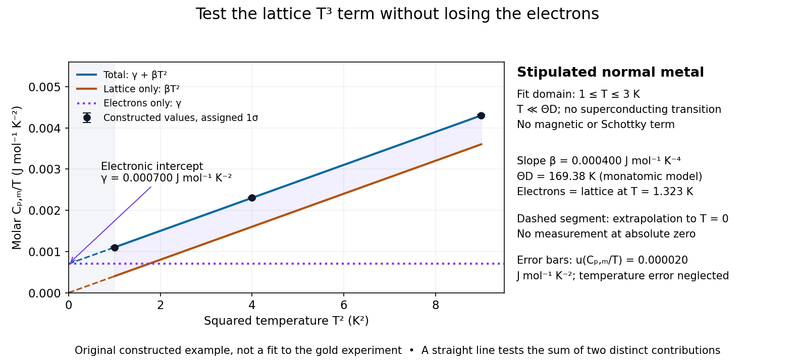

For a worked original inference, stipulate values of equal to at . Assign independent and negligible temperature error. Equal-weight linear regression on givesThe points sit exactly on the stipulated line; these standard uncertainties come from the assigned input precision, not an estimate from zero residual scatter. With , inversion givesAt , the electronic and lattice molar heat capacities are respectively and . Their equality occurs at : even in this clean model, the total heat capacity approaches a linear, rather than cubic, law as tends to zero in the normal state.
A straight line over a narrow interval is a useful diagnostic, not a universal proof. Inspect residuals and repeat the fit over several upper and lower temperature cutoffs; curvature can signal higher lattice terms, an unremoved Schottky anomaly, or a faulty calorimeter addenda subtraction. Correlated thermometer calibration and sample-amount errors affect both axes and can dominate the illustrative linear regression uncertainty. Low-dimensional samples, additional low-energy excitations and proximity to a phase transition need other models. The test is valuable precisely because its failures can reveal physics beyond the bulk acoustic approximation.
Low-temperature heat capacity measurement Created 2026-10-18 Updated 2026-10-20
Low-temperature calorimetry measures a small sample's heat capacity by resolving a small temperature change after a known electrical energy input. The experimental challenge is that the support, heater and thermometer also warm up. Their calorimeter addenda must be removed before interpreting the sample's phonons or electronic heat capacity. The Debye T-cubed test turns the corrected response into a test of the low-temperature vibrational spectrum.
Manuel Brando's 2009 experiment used a sapphire platform suspended by four alloyed platinum wires from a copper ring fixed to a cryostat stage. Grease attached the sample; a chip heater and ruthenium-oxide resistance thermometer served platform PLS-2. A controller stabilized the bath; a lock-in amplifier supplied heating pulses and read the calibrated sensor. The steady rise calibrated thermal conductance as . A separate , pure gold sample, compared with reference heat capacities, established the calorimeter addenda. Small pulses limited property variation; imperfect sample contact required a second relaxation time. The platform contribution rose below , making simple extrapolation unsafe.[ref]
Development of a Relaxation Calorimeter for Temperatures between 0.05 and 4 K by Manuel Brando. Brando, Development of a relaxation calorimeter for temperatures between 0.05 and 4 K, §§II–IV.B, Table I, Figs. 4, 5 and 8: construction, calibration, contact correction and low-temperature platform upturn
For an original idealization, assume sample and platform share one temperature , the bath remains at , and both the total heat capacity and the weak-link thermal conductance are approximately constant across one small pulse. Ignore other heat transfer and any phase transition. The first law of thermodynamics becomesHere is sample heat capacity, is calorimeter addenda, is deposited electrical power from Joule heating, and is a time constant. This is the same balance as calorimeter heat-loss correction, used here with a deliberately weak cryogenic link and a separately subtracted platform. For a constant pulse beginning at bath temperature, then switched off at ,The cooling exponential decay determines , while the heating plateau determines . Together with calorimeter addenda, they give . Cooling alone determines a ratio, not an absolute heat capacity. With finite , the observed end rise is smaller than the plateau; fit the full response or apply the displayed correction rather than identifying the two.
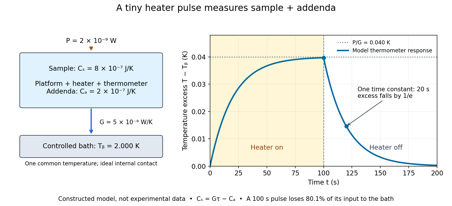

For the stipulated figure parameters, , , and give . The asymptotic rise is , only of bath temperature. At , the rise is . Of input, only remains stored: the other has flowed to the bath. Treating this long pulse as an isolated experiment would overestimate total heat capacity by a factor of .
Suppose independent standard uncertainties are , and . First-order propagation of uncertainty givesThe uncertainty is one standard deviation under those assumptions, about of sample heat capacity. Shared thermometer calibration errors can correlate fitted and ; then their covariance contributes too. Smaller samples amplify the relative influence of calorimeter addenda. Proposed checks include varying pulse amplitude, repeating with a reference sample, checking sensor self-heating, and comparing single- and two-time-constant fits. A drifting bath, slow internal equilibration or a transition invalidates this simple reduction even if a cooling curve looks smooth.
Regulated calibration bath 2026-10-18
A regulated bath holds its temperature near a chosen setting through feedback control, while stirring reduces internal temperature gradients. Its finite heat capacity buffers disturbances; external heating and cooling replace the ideal heat bath's unlimited capacity. This is useful for thermometer calibration and for maintaining a blackbody calibration source at a known temperature.
Joel B. Fowler's A Third Generation Water Bath Based Blackbody Source reports a NIST test of a stirred water bath containing a copper blackbody cavity. A bottom plate supplied heating and cooling; a double stirrer circulated water. Electronic feedback control regulated heating. An electronic thermometer with a thermistor probe provided the readout. The preparation was to approach a selected setting, wait for stabilization, adjust against the measured temperature and then log continuously.[ref]
A Third Generation Water Bath Based Blackbody Source by Joel B. Fowler. A Third Generation Water Bath Based Blackbody Source, §§2–3, printed pp. 592–593: bath construction, controller and setpoint procedure
To test spatial uniformity, one thermistor stayed near the cavity tip while another visited ten locations at three heights. The simultaneous reference distinguished spatial differences from temporal drift. An insulated dome reduced thermal conduction along probe casings. Table 1 reports nonzero departures at several settings: circulation did not make every location identical. The measurement uncertainty analysis separately included uniformity, stability, setting, immersion and readout contributions. These tests supported a bounded temperature assignment around the cavity, rather than infinite heat capacity or perfect thermal equilibrium throughout the apparatus.[ref]
A Third Generation Water Bath Based Blackbody Source by Joel B. Fowler. A Third Generation Water Bath Based Blackbody Source, §4.1 and Tables 1–2, printed pp. 594–595: fixed and movable probes, immersion control, measured nonuniformity and uncertainty components
Finite heat bath 2026-10-18
A finite heat bath has a finite whole-body heat capacity and therefore changes temperature when it absorbs heat . For a rigid closed system with no work, fixed composition and no phase transition, the first law of thermodynamics givesIf the heat capacity at constant volume is constant throughout this temperature interval, the integral becomes . This statement concerns an internal energy difference; need not be the body's absolute internal energy.
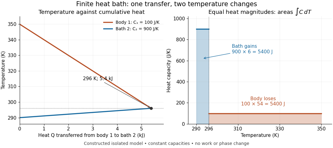
For an original example, put a rigid body 1 and a finite bath 2 into thermal contact inside an isolated system. Stipulate constant whole-body heat capacities and , with initial temperatures and . Each body remains internally uniform; the connection stores negligible energy; no external work, matter exchange or phase transition occurs. These are constructed model values. The argument in thermal equilibration of two finite bodies applies directly: equal final temperatures and conserved total internal energy giveThus the heat transferred from body 1 to bath 2 isBody 1 loses of internal energy and bath 2 gains exactly that amount. Body 1 cools by , while bath 2 warms by . Equal heat transfers produce unequal temperature changes because the heat capacities differ.
Finite bath temperature changes and the integrated heat ledger
. Original constant-heat capacity model, not measured data. Left: accumulated heat leaving body 1 lowers its temperature and raises bath 2's temperature; the lines meet at and . Right: the shaded integrals have equal area , although their widths are and . The outgoing heat magnitude is shown positive; body 1's signed internal energy change is negative. Details.
The heat bath approximation can now be assessed against a chosen allowed temperature change . Constant requires , rather than merely calling the bath large. For this example, an allowed change of would fail because the computed change is . The exact bath shift and its ideal-reservoir limit areHold and both initial temperatures fixed in this limit. The transferred heat then approaches . The finite bath receives less heat because its warming reduces the available temperature difference. For heat capacities that vary, use the two integrals in the energy balance instead of this weighted average.
Conservation of energy also permits imagining the reverse transfer, so it cannot explain the direction of equilibration by itself. Entropy from heat capacity gives the additional test, using reversible comparison paths between equilibrium endpoints:All ratios inside the natural logarithms use absolute temperatures. The actual exchange across unequal temperatures is irreversible, even though reversible paths calculate the endpoint entropy differences.
There is a short general proof of positivity. Put for positive constant heat capacities and positive initial temperatures. The strict concavity of the natural logarithm giveswith equality only for equal initial temperatures. In this proof all temperatures inside the logarithms mean their numerical values in one common absolute unit. This is Jensen's inequality applied to the same weighted average that conservation of energy selected. The direction of heat transfer and the stability of its endpoint also follow from entropy maximization under thermal contact.
Photon-number measurement backaction 2026-10-18
An explicit original ideal meter model explains how photon number survives while field quantum coherence changes. Let be the number operator and prepare an atomic qubit in . The dispersive unitary operatorcommutes with . For a field quantum superposition , it produces , where . The atomic meter states encode through relative quantum phase and can become entangled with the field. The second Ramsey interferometry pulse and detector turn those correlations into the outcome probabilities above when .
Tracing out the atom multiplies a field density matrix entry by . Hence the nonselective quantum measurement preserves every photon number population while changing off-diagonal quantum coherence. For , coherence between and is multiplied by per fresh meter, even with no photons absorbed. Field quantum phase information can therefore be disturbed by an energy-preserving probe. No universal self-adjoint phase operator or naive canonical number–phase commutator is needed for this conclusion.
One possible finite-contrast quantum instrument makes the distinction sharper. Define diagonal Kraus operators and . After their ideal readout, flip the reported label with probability . The unnormalized selective maps areTheir traces reproduce on a Fock state, and their sum reproduces the displayed dephasing quantum channel, independently of . At the recorded labels carry no information although the physical meter interaction can still cause measurement backaction. This is an illustrative instrument, not a reconstruction of all laboratory imperfections; equal likelihoods alone do not determine the disturbance.
Sequential Bayesian photon counting 2026-10-18
Consider an original balanced-readout model, rather than a fit to the experiment. Let , with a normalized prior probability and . A detected chemical atom has outcome . Define the conditional probabilitiesHere is the accumulated quantum phase per photon, the controlled analysis quantum phase, and the fringe contrast. The two probabilities sum to one for every . Actual calibration may also require an offset and asymmetric detection errors; alone does not specify a quantum instrument.
Assume no photon number change during the record and fresh independently prepared atomic meters. For observed outcomes at recorded settings , the Born rule and Bayes' theorem giveThe posterior probability is defined only for . Summing its numerator over proves normalization. This is also the update of diagonal elements of a field density operator under a measurement in quantum mechanics; it does not assume that an initial quantum superposition was an unknown pre-existing integer. The observed settings are part of the record, especially when selected adaptively.
For an exact finite example take , , and . An outcome at has likelihood , giving . Another at gives . A subsequent at givesThus three atomic records raise the posterior probability of from to , while leaving finite uncertainty. No one of these outcomes identifies with certainty.
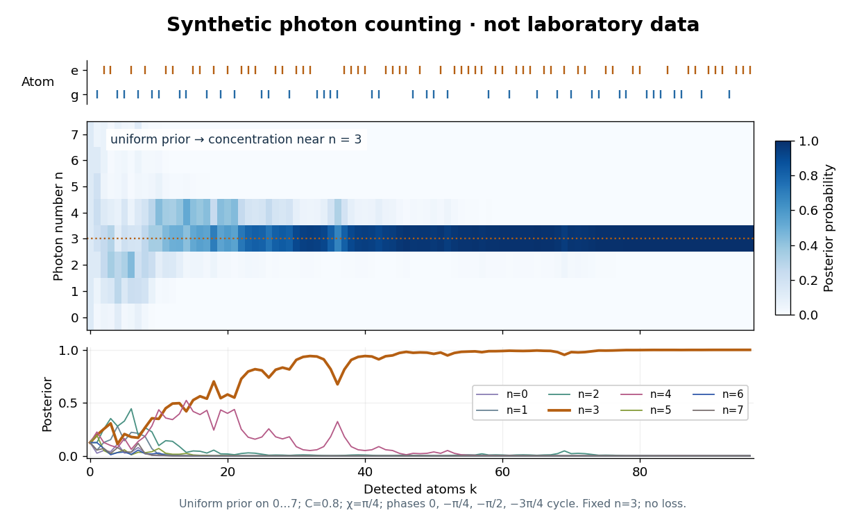

The periodic likelihood function imposes an identifiability limit. If for an integer , then for every setting: the posterior odds between and never change. Varying can resolve a cosine reflection ambiguity within a period, but cannot remove this exact period. Changing can supply additional information. A finite cutoff is therefore a physical assumption to justify, not evidence that excluded high photon numbers were absent. At no outcome changes the prior probability; at neither binary outcome has an exactly zero likelihood.
The no-loss assumption also has a time limit. In an original zero-temperature loss model, let . A Fock state loses its first photon at rate , so its survival probability is and its mean lifetime is for . Several records must be acquired within that lifetime to identify a plateau. When losses matter, first predict using a normalized transition matrix, then apply the atomic Bayesian inference update to . Thermal excitation requires upward transitions too. A delayed or broadened inference after a jump need not indicate that an atom caused the jump.
For a holomorphic function , the Cauchy-Riemann equations imply and . At a point where , the two regular level curves therefore meet at right angles, since each tangent is perpendicular to its nonzero gradient. The noncritical condition is necessary: for , the zero level sets are the coordinate axes and the two diagonals, which meet at angles of at the critical point zero. Orthogonality at regular points is one geometric expression of conformality.
Cold-atom realization of the Haldane model 2026-10-18
Gregor Jotzu and collaborators realized an artificial Haldane model in 2014. They loaded spin-polarized potassium-40 fermions into a laser-made honeycomb lattice. Piezoelectric mirrors shook the optical lattice along two axes; their relative phase controlled time-reversal symmetry breaking. Optical phase control adjusted the sublattice offset.[ref]
A magnetic field gradient drove Bloch oscillations. Band mapping measured interband transfer to locate valley-gap closures. Opposite-force drift measurements distinguished cancelling from reinforcing Berry curvature contributions; reversing shaking handedness reversed the drift. Interband transfer and harmonic confinement affected this readout, including drift beyond ideal transition lines. This neutral-atom Floquet Hamiltonian realization did not measure electrical sheet conductivity. Magnetic fields were used for preparation and forcing.[ref]
Chern number of the Haldane model 2026-10-18
For , put . The lower-band orthogonal projector is . Applying the Pauli matrix multiplication law to givesThus the Chern number is the signed number of times the Brillouin zone covers a two-sphere under . The lower energy eigenstate's actual Bloch vector is . The Berry curvature has the displayed positive sign for this lower band and the stated Berry connection; switching to the upper band changes its sign.
A useful local calculation exposes what each valley contributes. Write . The linear Dirac Hamiltonian givesEach unbounded continuum cone gives a half-integer in this calculation. It is not a separately realizable half-integer Chern number of an isolated lattice energy band. The full honeycomb lattice supplies both valleys and the large-momentum completion. Starting with a trivial large- state, each single-valley mass crossing changes the lattice integer by the corresponding unit. There are no other band touchings. This establishes the exact lattice resultfor , excluding the boundaries. This sign belongs to our explicit bond vectors, orientation and occupied-band convention.
For an original worked example, choose , , and . Then , , both valley gaps are , and . Choosing instead , gives exactly the same valley-gap magnitudes but . The first state's two valley contributions reinforce; the second state's cancel.
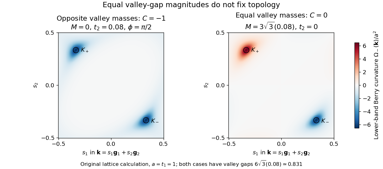
Equal valley gaps can conceal different Berry-curvature topology
. Original calculation of the lower-band Berry curvature of the two explicitly defined lattice Hamiltonians, using the same colour scale. One reciprocal primitive cell is shown in fractional coordinates, with , , and . The bond length is . The coloured surfaces are model results, not measured curvature or a reconstruction of experimental data. Source. Details.
An independent eigenvector-overlap calculation on periodic , and momentum grids gives for the first example and for the second. Reversing in the first example gives . Direct integration of the analytic lattice Berry curvature agrees. For the overlap calculation one can remove the embedding phase from , replacing it by ; this makes the cell-basis Hamiltonian periodic and prevents a false boundary-seam contribution. The local Berry curvature can depend on this basis convention; the integrated Chern number agrees. All mass-zero parameters are excluded before evaluating any integer.
Valley masses of the Haldane model 2026-10-18
The only zeros of , modulo the reciprocal lattice, are the two Dirac valleys in graphene,At these momenta . Thus the two Dirac mass coefficients, measured in energy units, are , with . For ,The two Dirac cones have opposite orientation, encoded by . A scalar sublattice offset gives equal-sign Dirac masses; imaginary second-neighbour hopping at gives opposite-sign Dirac masses. Both mechanisms open valley gapsAn observed band gap alone therefore cannot establish a Chern insulator. In particular, the gapless nearest-neighbour model of graphene and its sublattice-mass deformation should not be confused with the topologically nontrivial Haldane model.
A band gap closes when all three components of vanish. Since only at the two valleys, the phase boundaries are exactly . Usually one valley becomes massless; at , , both do. The occupied-band Chern number is undefined at every such touching, even if a numerical momentum grid misses its location.
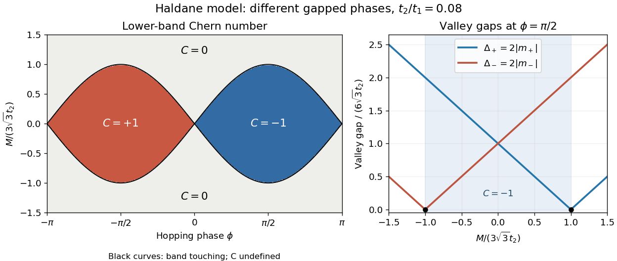
Haldane phases meet where a valley gap closes
. Original model calculation with the stated lower-band Berry-connection convention and . Left: integer Chern numbers; black curves denote singular parameters, where no Chern number is assigned. Right: the two valley gaps along ; the vertical axis shows valley gaps, rather than an assumption about global band extrema. No experimental data are plotted. Source. Details.
There are unlisted articles, also show them or only show them.