
Gargamelle Created 2026-10-18 Updated 2026-10-20
Gargamelle was a heavy-liquid bubble chamber at CERN. Its 1973 collaboration report, Observation of neutrino-like interactions without muon or electron in the Gargamelle neutrino experiment, by F. J. Hasert and colleagues, described hadronic events with no identified muon or electron and evaluated rates relative to charged current events. This is evidence for a neutral current, rather than direct production or photography of a Z boson.[ref]
Observation of neutrino-like interactions without muon or electron in the Gargamelle neutrino experiment by F. J. Hasert. Physics Letters B 46 (1973), pp. 138–140, title, abstract and author list
CERN's Gargamelle account identifies the target liquid as and distinguishes hadronic events from the separate isolated-electron signal. The latter is an antineutrino transferring momentum to an electron, whose electromagnetic particle shower supplies visible tracks. These are different final states, not two names for one event.[ref]
Forty years of neutral currents by Cian O’Luanaigh. Forty years of neutral currents, 19 July 2013, chamber description and isolated-electron caption
A neutrino beam uses protons striking a target to produce charged pions and kaons; focusing selects parents that undergo particle decay in flight. Their neutrinos pass through shielding into the target. Scanning photographs locates vertices and classifies outgoing tracks.[ref]
Expansion prepares a bubble chamber's superheated liquid; ionization by charged secondaries seeds bubbles for photography.[ref]
The recorded light reveals bubbles, not a directly visible incoming or outgoing neutrino. Reconstructing a vertex and classifying bubble-chamber tracks connects that optical record to a hypothesis about a particle interaction.
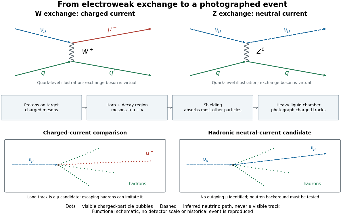
The collaboration compared samples with matched hadronic cuts. A flat longitudinal vertex distribution resembled neutrino interactions, but sideways neutrons and multi-step cascades could also flatten it. The background estimate combined visible parent-interaction/secondary-neutron pairs with a cascade calculation including surrounding material. Later proton exposures tested the predicted cascade lengths. Escaping charged hadrons could imitate muons; there was no independent perfect muon tag.[ref]
The inference combines positive evidence for an interaction with controlled alternatives for its visible final state. Shielding suppresses unwanted beam components, yet interactions in surrounding material can generate secondary neutrons; shielding alone cannot certify a neutral current. Nor does a successful neutral current search by itself establish every coupling or the Higgs mechanism. Its importance for the electroweak interaction is that the theory predicts an additional weak channel, with coupling relations that further cross section measurements can test.
Dirac valleys in graphene Created 2026-10-18 Updated 2026-10-20
At either displayed wave vector, the three complex hopping amplitudes add to zero: . Therefore the energy bands touch. There are two inequivalent electronic valleys; other equivalent corners are related by reciprocal-lattice translations. Setting and retaining first-order terms giveswhere are Pauli matrices. For example, at , . The matrix has the form of a massless two-dimensional Dirac Hamiltonian. Here is a material-model velocity, rather than the vacuum speed of light; this description does not change an electron's vacuum rest mass. It describes the dispersion relation of electronic excitations near a band crossing.
Rayleigh stability integral identity 2026-10-18
Multiply the narrow-gap centrifugal stability equation by the complex conjugate mode and use integration by parts with zero endpoint radial velocities. This gives the displayed real Rayleigh quotient. Its denominator is positive. Positive Rayleigh discriminant throughout the gap gives positive for every nonzero mode, excluding exponential axisymmetric growth; nonnegativity permits marginal cases. In the alternative convention , the numerator is , so the stable sign is . For rigid rotation, gives .
Glucose mutarotation experiment 2026-10-18
An endpoint experiment uses a polarimeter with a sample cell and supplied , and D-glucose chemical solutions. Collect about of each. Fill the cell first with distilled water, dry its windows, move bubbles to the air trap, and retain its orientation. Scan light intensity against polarimeter analyzer angle through . The protocol fits a Gaussian function to the upper third of a symmetric peak to locate its maximum. Rinse with the next sample, repeat for each glucose chemical solution, and subtract the water maximum's angle from each sample maximum. This is an operational peak-location method; the Gaussian function is not the physical transmission law.[ref]
Equilibrium of Sugar Mutarotation by PASCO. PASCO, Equilibrium of Sugar Mutarotation, p. 1 path length; pp. 2–4 Materials and Equipment and Procedure 1–18
The existing optical activity and polarimetry articles explain the apparatus, Malus's law and instrument limitations. For an extension that observes mutarotation in time, freshly dissolve a specified crystalline anomer, record the mixing time, and repeat the optical rotation readout at fixed concentration, path length, wavelength and recorded temperature. Keep pH consistent and record the delay before the first reading. These are proposed additions to the endpoint protocol, not its published steps or a claim of measured results. Recheck the water blank, repeat the preparation, and compare with a separately equilibrated portion under the same conditions. A stable endpoint alone does not show the time evolution.
Interpret each concentration separately. If is blank-corrected optical rotation, is path length and is total glucose mass concentration, first calculate specific rotation . In an additive two-anomer approximation, let be reference specific rotations under the same conditions and the mole fraction of alpha within that pair. Equal molar masses make its mass fraction equal to , soThis is a population estimate from an assumed response model, not direct imaging of an anomer. For a simple consistency check, doubling at fixed and unchanged composition doubles in this model while leaving unchanged. Averaging raw optical rotations at different concentrations would fail this test; normalize first.
Changing temperature, pH, contamination, incomplete dissolution, window stress, bubbles or instrumental drift can imitate or obscure a changing signal. Reference specific rotations must match the sample conditions. Minor open-chain and other ring forms limit the two-anomer approximation; a single optical rotation cannot separately determine every population. Also, these anomers are diastereomers, not an enantiomer pair: the equal-and-opposite cancellation formula for enantiomeric excess does not apply.
Spatial resolution from momentum transfer Created 2026-10-18 Updated 2026-11-05
In quantum scattering, a spatial feature on scale contributes Fourier components with wavenumber of order . A momentum transfer of magnitude supplies wavenumber , giving the characteristic estimate . With the energy-like quantity , this becomes . The full de Broglie wavelength uses and differs from the corresponding reduced wavelength by . Beam energy only bounds accessible momentum transfer; it does not determine the resolution of every event.
Mode-locked laser Created 2026-10-18 Updated 2026-11-05
A mode-locked laser maintains definite relative wave phases among many longitudinal resonator modes. Their coherent sum forms a repeating train of short optical pulses, rather than merely producing a broad optical spectrum.
For an ordinary linear resonator, the repetition interval is approximately the round-trip travel time. More phase-aligned spectral bandwidth permits shorter pulses, subject to the time-bandwidth product and spectral shape. A photodetector can measure pulse-train timing, while an intensity autocorrelation estimates much shorter pulse durations under a stated model. Neither a broad spectrum nor a fast periodic intensity signal alone uniquely reconstructs the pulse's complex electric field.
Uniform distribution with an atom at zero Created 2026-10-18 Updated 2026-10-20
For and , this mixed probability distribution has probability mass at zero and ordinary probability density function on . That ordinary density integrates to , not to one; conditioned on , the law is the uniform distribution on . Its cumulative distribution function is zero for , for , and one for .
For each positive integer , integration gives . Thus the expected value is and the variance is . The nonzero atom contributes to normalization even though it contributes zero to positive moments. At , conditioning on positive delay is undefined because the conditioning event has probability zero.
For a matched receiver accepting one spatial mode and one polarization of waves, the thermal contribution to the available spectral power of a blackbody isThis expression excludes a zero-point term; it is the thermally emitted contribution. Defining the Rayleigh-Jeans law equivalent antenna temperature by gives the displayed relation. With ,Thus requires . It is an approximation with a frequency-dependent error, rather than a redefinition of thermodynamic temperature.
For the stipulated and , and . Replacing by here would differ by about . At much higher frequencies, the approximation fails more strongly. A real instrument averages over its measured frequency response and antenna beam pattern, so using a single central frequency adds a narrow-band approximation.
Protease protection assay 2026-10-18
A protease protection assay asks whether a barrier prevents an added protease from reaching a protein. A membrane-disruption comparison tests whether protection depends on that barrier.
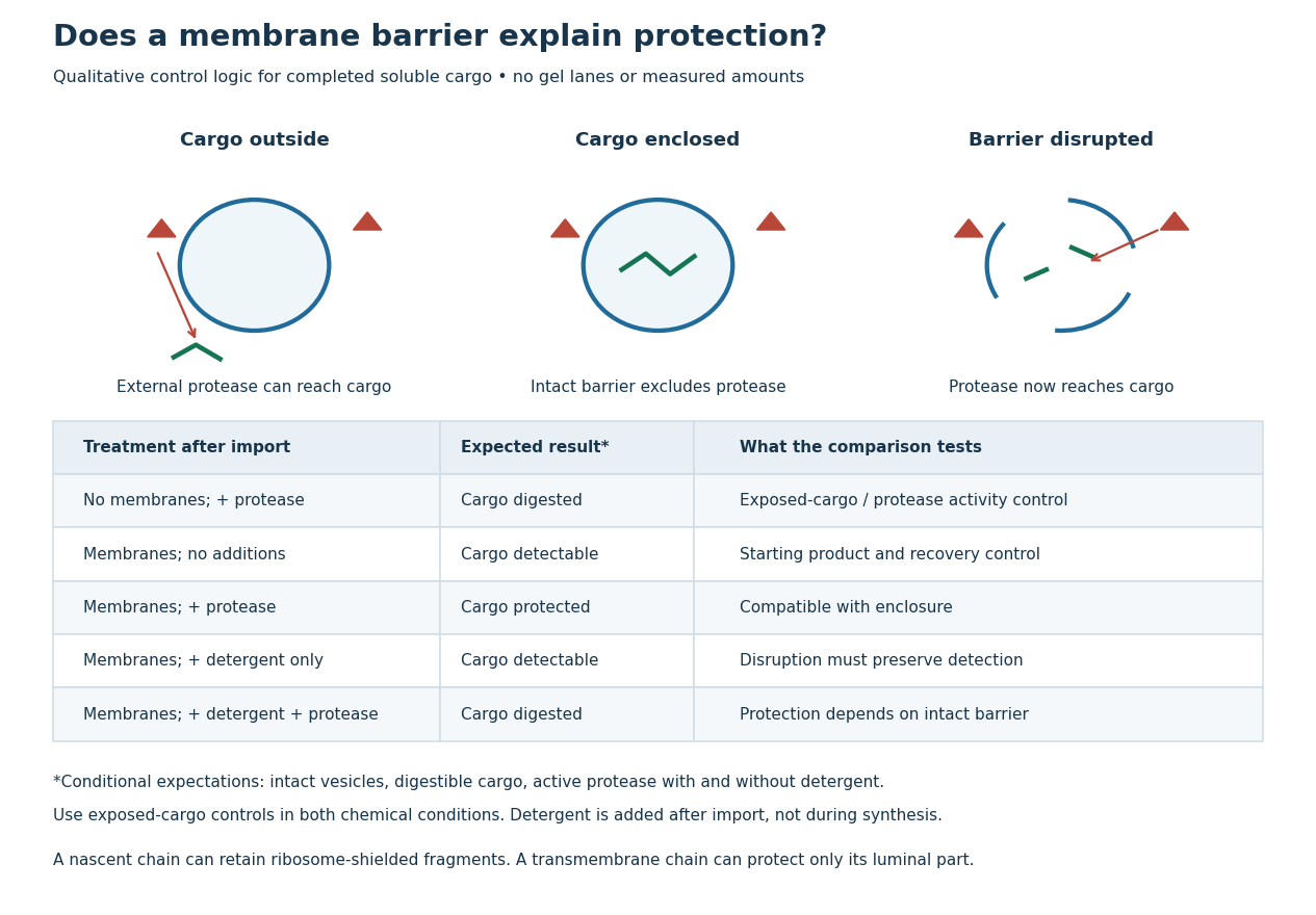
Protease protection assay: accessibility and control logic
. Original qualitative decision diagram for a completed soluble cargo. Icons and words describe expected outcomes under stated assumptions; they are not an autoradiography readout, copied historical lanes, measured survival fractions or simulated experimental intensities. Detergent is added after the import reaction. The historical nascent chain experiment also retained small ribosome-protected fragments, which this completed-cargo model deliberately distinguishes. Details.The membrane-disruption test was performed by David D. Sabatini and Günter Blobel in 1970. Rat-liver microsomes purified by sucrose centrifugation incorporated radioactive leucine during cell-free translation. Samples received cold trypsin and chymotrypsin, with or without membrane-solubilizing detergents. Electron microscopy checked vesicle preservation; size-exclusion chromatography separated protected fragment sizes. Large membrane-associated fragments lost protection after disruption, whereas small ribosome-protected fragments persisted. An exposed ribosome preparation remained digestible when mixed with microsomes, checking that membranes did not simply inhibit the proteases.[ref]
Controlled Proteolysis of Nascent Polypeptides in Rat Liver Cell Fractions II by David D. Sabatini and Günter Blobel. Controlled proteolysis of nascent polypeptides in rat liver cell fractions. II, Methods p. 147; activity control p. 148; Figure 5C–D and text p. 152; Discussion pp. 155–156
To read the qualitative diagram, first compare untreated aliquots: they establish that detectable cargo exists before digestion. Next compare external protease with intact versus disrupted membranes. Persistence only while the barrier remains intact supports enclosure, provided the exposed-cargo control confirms active protease in both chemical conditions. The detergent-only aliquot checks that disruption itself does not destroy recovery or detection. Adding membranes after synthesis tests a different alternative: capture of a completed product rather than entry during biological translation.
This is an argument from controlled accessibility. Binding predicts membrane association but generally leaves an exposed cargo digestible. Enclosure predicts protection that depends on membrane integrity. However, protein aggregation, intrinsic resistance to proteolysis, inactive protease or undetected small fragments can obscure this distinction. For a transmembrane protein, expect protection of the enclosed portion rather than necessarily the full chain. Combine fragment size, compartment controls and membrane topology; a protected signal alone does not uniquely specify the whole protein's location.
Cutoff frequency of a membrane waveguide 2026-10-18
The cutoff frequency of a membrane waveguide is the lowest frequency at which a specified transverse normal mode can propagate longitudinally. For fixed edges separated by , and . Below cutoff the longitudinal wavenumber is imaginary and a bounded excitation is an evanescent wave. Above it, and .
Bending stiffness in a membrane waveguide Created 2026-10-18 Updated 2026-10-20
For a plate under uniform tension per length , with surface mass density and flexural rigidity , the small-displacement equation is . If the edge conditions admit a transverse sine mode of wavenumber , its longitudinal dispersion relation isBending raises mode cutoff frequencies of a membrane waveguide and changes large- behaviour from to . A genuinely clamped plate also fixes the edge slope, so its transverse mode shapes need not remain simple sine functions. The qualitative increase in restoring force survives that change of boundary conditions.
For a finite list of real values , maximize information entropy with , , and . Lagrange multipliers giveThe constrained second variation is for any nonzero tangent perturbation, proving uniqueness of the entropy maximum whenever a feasible interior solution exists. The mean has derivative , so for nonconstant it decreases strictly with and ranges between the largest and smallest as ranges over the real line. Thus a finite exists uniquely exactly when .
At an extreme mean, strictly positive probabilities are impossible unless all coincide. If all , the mean constraint is redundant when , the maximum is uniform, and is not identifiable. This finite exponential family is an exponential tilting of the uniform distribution.
Preconditioned steepest descent Created 2026-10-18 Updated 2026-10-31
For fixed symmetric positive-definite matrices and , preconditioned steepest descent minimizes along the direction supplied by the auxiliary solve. Given , form the linear-system residual . If , stop: . Otherwise solve and useThis is exact line search for a positive-definite quadratic along . Indeed,whose derivative vanishes at the displayed positive step size. Unlike the Preconditioned conjugate gradient method, it uses the fresh directly rather than combining it with a previous conjugate direction.
For diagonal scaling for a two-dimensional linear system, start at . Without matrix preconditioning, take : , , andWith the Jacobi preconditioner , , , andThe original linear-system residual becomes much smaller after this correction. Quantify progress in the same energy norm in both cases: and . Exact substitution givesIn this particular example the entire histories are and . To check that this is exact, the next step sizes are and , respectively, and their residual updates give and . Multiplying a linear-system residual by a nonzero scalar leaves the next step size unchanged; every pair of steps repeats the same directions at a smaller scale. The two first-step energy ratios then establish these formulas for all .
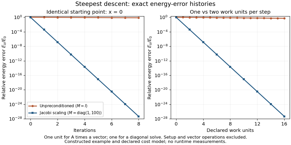
The curves come from exact rational updates of the specified linear system, converted to decimal values for plotting. The left panel counts iterations. The right panel declares one unit for applying and one unit for the auxiliary diagonal solve, charging one unit per unpreconditioned step and two per preconditioned step. It excludes setup and vector operations, so it compares a declared cost model rather than measured runtime. Scaling is advantageous even with that extra charge.
These curves compare steepest descent method iterations. On this two-dimensional linear system, both the conjugate gradient method and the Preconditioned conjugate gradient method terminate within two steps in exact arithmetic. The plot therefore establishes no CG iteration-count advantage for this example; the benefit of scaling for larger problems depends on their eigenvalues and auxiliary-solve costs.
Consider the original linear systemCompleting the square proves that is a symmetric positive-definite matrix:The Jacobi preconditioner has . Symmetric positive-definite preconditioning givesIts eigenvectors and have eigenvalues and . HenceThe characteristic polynomial of is . Its eigenvalues and spectral condition number of a positive-definite matrix areThe ellipse axis ratio drops from about to . The transformation multiplies the second coordinate by ten, bringing the two energy scales together.
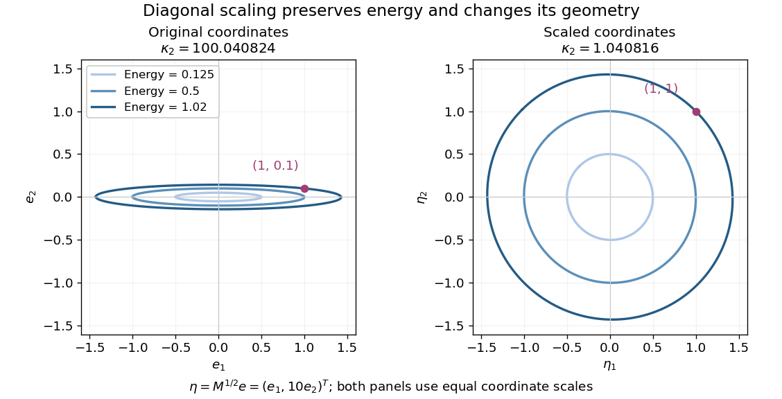


Both panels show the same energy level sets, expressed in error coordinates and . Their coordinate axes have equal scales. The marked displacement becomes ; its energy remains . These are exact contours of the specified quadratic form.
Solving the original equations givesDirect matrix multiplication checks both linear-system residuals:By contrast, left preconditioning gives , which is visibly not a symmetric matrix, despite having the same positive eigenvalues as .
A bad scaling can reverse the benefit: the still valid symmetric positive-definite matrix gives . Its Rayleigh quotients on the coordinate unit vectors are and , so . Cheapness and positive definiteness do not guarantee improved conditioning.
Symmetric positive-definite preconditioning Created 2026-10-18 Updated 2026-10-31
Let and be real symmetric positive-definite matrices. The principal square root of a positive semidefinite matrix construction gives an invertible matrix for each. SetThen is equivalent to . This is a matrix congruence, and is a symmetric positive-definite matrix: , and for every nonzero vector ,since . This short proof establishes both requirements for applying the conjugate gradient method to the transformed linear system.
The left transformed matrix has the same eigenvalues becauseIts correct geometry uses the weighted inner product : . Thus it is symmetric in this inner product, even when it is not a symmetric matrix in ordinary coordinates. The spectral condition number governing the transformed symmetric problem is , not generally .
The Preconditioned conjugate gradient method realizes this transformation using auxiliary solves , without constructing or its matrix inverse. With fixed , initialize and ; while , usethen solve and setStop at a zero linear-system residual before forming another ratio. Positive definiteness makes the denominators positive before termination.[ref]
Notes for Ma221 Lecture 15, Dec 1, 2023. Math 221, Matrix Computations, Fall 2023; Notes for Ma221 Lecture 15, Dec 1, 2023; PDF p. 1, equivalent symmetric system and Preconditioned CG algorithm
An invertible matrix alone is insufficient: with and , the left transformed matrix has eigenvalues , and has no real symmetric positive-definite matrix square root. Even a valid symmetric positive-definite matrix can worsen conditioning if its scaling is unsuitable, as the next worked example shows.
Right preconditioning 2026-10-18
Right preconditioning substitutes into the linear system . Applying its transformed linear map first solves , then computes . Recover the solution by solving . Its linear-system residual is exactly the original linear-system residual , which is useful when monitoring the imbalance in the original equations.
The left preconditioning and right preconditioning transformed matrices are similar matrices:They therefore have the same eigenvalues, although their Euclidean norm condition numbers and residual histories need not agree. A similarity transformation preserves eigenvalues; a nonorthogonal change of coordinates need not preserve lengths.
Left preconditioning Created 2026-10-18 Updated 2026-10-31
Left preconditioning multiplies both sides of the linear system by the same invertible matrix . It leaves the unknown vector unchanged. The original linear-system residual is ; the transformed linear-system residual is . Applying the transformed linear map to first computes , then solves .
For symmetric positive-definite matrices and , is generally not a symmetric matrix in the Euclidean inner product. Its positive eigenvalues alone do not justify ordinary Euclidean conjugate gradient method recurrences. The remedy is symmetric positive-definite preconditioning, implemented through the Preconditioned conjugate gradient method.
Matrix exponential respects similarity Created 2026-10-18 Updated 2026-11-05
For an invertible matrix , induction gives , including . The power series for the matrix exponential is absolutely convergent in every matrix norm, so multiplication by the fixed matrices can be taken through the sum. This proves the displayed identity without any diagonalizability assumption. In particular, if with diagonal, then .
Exponential of a skew-Hermitian matrix 2026-10-18
If is Skew-Hermitian, then is a Hermitian matrix. The finite-dimensional spectral theorem gives , with real and a unitary matrix . Since the matrix exponential respects similarity, . Each diagonal entry has modulus one, so is a unitary matrix. Thus a skew-Hermitian matrix generates norm-preserving linear evolution.
Exponential of a Hermitian matrix 2026-10-18
A Hermitian matrix has a unitary spectral decomposition with real eigenvalues . The matrix exponential respects similarity, giving . Its eigenvalues are positive and its conjugate transpose equals itself. In particular for , so it is a Hermitian positive-definite matrix.
There are unlisted articles, also show them or only show them.