
Matrix inverse from a decaying matrix exponential Created 2026-10-18 Updated 2026-11-05
If every eigenvalue of a finite square matrix has negative real part, its matrix exponential decays and its integral converges. The Jordan normal form shows that polynomial factors in are dominated by exponential decay. Integrating gives , proving the displayed matrix inverse formula. In particular, for a Hermitian matrix with negative eigenvalues, the spectral theorem reduces the integral to scalar exponentials with integrals . The minus sign is essential: the integral is positive definite in this Hermitian case, while has negative eigenvalues.
Maser oscillation threshold 2026-10-18
The following original model isolates amplification by inverted electric dipoles. Let be the excess number in the upper member of one equally degenerate resonant pair. Let be a slowly varying cavity amplitude with photon number , and let describe the collective molecular dipole component in the amplifying phase convention. On exact resonance, stipulate the linear equationsThe dipole relaxation rate is , and is a single-molecule coupling in the chosen mode normalization. Here is an electric dipole moment matrix element, is the field's zero-point amplitude, and . Field overlap and dipole orientation enter this coupling. The characteristic polynomial for growth rate isFor , one root becomes positive precisely when . If dipole relaxation is fast enough to eliminate , then andThus positive population inversion alone is insufficient: the gain rate must exceed the passive decay rate. This reduction describes the onset near resonance; it does not predict output phase noise, actual transit dynamics or an exact historical threshold. Nikolay Basov and Aleksandr Prokhorov's molecular-generator theory likewise treats self-excitation as competition between molecular gain and resonator-plus-load losses.[ref]
Theory of the Molecular Generator and Molecular Power Amplifier by Nicolay Gennadiyevich Basov and Aleksandr Mikhailovich Prokhorov. p. 426, Introduction; pp. 427–428, dipole response and self-excitation
To include replenishment, suppose upper-state molecules enter at rate and both levels leave with residence rate . A deliberately simple ordinary differential equation model isOne downward transition removes two units of the difference , so . Below onset the unsaturated inversion is , givingFor fixed mode volume , the equivalent number density condition is . Raising selected beam intensity raises gain; increasing quality factor lowers the loss rate at fixed frequency. These statements hold with , residence time and mode overlap fixed.
Above onset, the nonzero steady state hasThe inversion is clamped while excess supply supports output. A finite initial seed is understood: the noiseless equations leave exactly unchanged even above onset. Actual startup has spontaneous emission and field fluctuations.
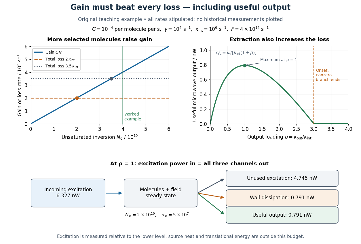
Maser oscillation threshold, output loading and the maser microwave energy budget
. Original illustrative model, not historical measurements. Left: gain rises with selected beam supply, crossing two chosen total loss rates. Right: with fixed supply, output initially grows with output coupling, then falls to zero when that coupling makes the total loss too large. The lower panel accounts for incoming excitation, unused excitation leaving in the beam, wall dissipation and useful output for the worked example. Details.
Saturation magnetostriction Created 2026-10-18 Updated 2026-11-05
In the saturated isotropic magnetostrictive strain convention, saturation magnetostriction is the longitudinal relative length change from a random-domain reference to alignment. A parallel-to-perpendicular length difference instead equals in that model.
Volume magnetostriction 2026-10-18
Volume magnetostriction is the relative volume change associated with a magnetic-state change. To first order it is the trace of the magnetostrictive strain. Zero trace is an additional restriction, not a consequence of isotropy alone.
Manganese monoxide neutron diffraction experiment Created 2026-10-18 Updated 2026-10-20
In 1949, Clifford Shull and J. Samuel Smart compared powdered manganese(II) oxide at room temperature and . Powder preparation supplies many crystal orientations. Their Fig. 1 records scattered-neutron intensity versus counter angle. Nuclear reflections remained, while the cold pattern gained strong reflections forbidden by the chemical unit cell. They indexed these with a magnetic unit cell having twice the chemical cell edge. The warm pattern already contained diffuse magnetic scattering: loss of sharp magnetic peaks does not mean loss of individual magnetic moments.[ref]
Detection of Antiferromagnetism by Neutron Diffraction by Clifford Glenwood Shull and J. Samuel Smart. Shull and Smart, Detection of Antiferromagnetism by Neutron Diffraction (1949), Fig. 1 and accompanying paragraphs; original reprint inspected at Carnegie Mellon University
The source was Oak Ridge's graphite-moderated reactor. In Early Development of Neutron Scattering (1994), Clifford Shull describes how the early two-axis instruments used a monochromating crystal to select the incident-neutron wavelength; a shielded neutron counter rotated around the specimen to record angular intensity. This specifies the source–monochromator–sample–counter path, without identifying which instrument revision produced the MnO trace.[ref]
Early Development of Neutron Scattering by Clifford Glenwood Shull. Early Development of Neutron Scattering (1994), pp. 99–103, Figs. 2–4, and p. 106, Fig. 8; inspected CMU reprint pp. 99–106
The control was the same compound above and below magnetic ordering, with retained nuclear peaks identifying the underlying chemical periodicity. The original paper labels an aluminium impurity peak and defers a complete magnetic-structure account. It supplies neither a chemical synthesis recipe nor detailed cold-stage construction. The inference is periodic magnetic order, rather than a claim that every possible structural change was excluded at arbitrary resolution.[ref]
Detection of Antiferromagnetism by Neutron Diffraction by Clifford Glenwood Shull and J. Samuel Smart. Fig. 1: aluminium impurity label, nuclear/magnetic indexing and room-temperature/80 K comparison; final paragraph before conclusion
The connection to the measured angle is the elastic Bragg scattering condition. If the incident and outgoing wave vectors have equal magnitude and make an angle , their difference has magnitudeA longer real-space period supplies additional, smaller reciprocal lattice spacings, which can put magnetic reflections at new counter angles. In the one-dimensional toy model above, doubling the period changes the allowed spacing from to . The actual MnO indexing is three-dimensional; the toy row does not assert its reflection positions or relative peak strengths.
Louis Néel supplied the ordering theory; the 1949 diffraction work was a later experimental test. His 1970 Nobel Prize in Physics recognized antiferromagnetism and ferrimagnetism. Clifford Shull's neutron-diffraction award followed in 1994.[ref]
The Nobel Prizes in Physics 1901–2000 by NobelPrize.org. sections on neutron diffraction and magnetic ordering: Néel 1970 and Shull 1994
Magnetic field of a rotating charged spherical body Created 2026-10-18 Updated 2026-11-05
A uniformly charged solid sphere of total charge , radius and angular velocity has magnetic dipole momentFor a uniformly charged thin spherical shell the coefficient is instead of . At large distances the magnetic field is a magnetic dipole field, . Its angularly averaged magnitude and root mean square magnitude both scale as ; its angularly averaged vector is zero. Steady rotation of this axisymmetric charge distribution produces magnetostatics, not radiation.
Magnetic dipole inclination versus latitude Created 2026-10-18 Updated 2026-11-05
For a centred magnetic dipole moment pointing toward geographic south, the field at northern latitude has northward component and downward component . These follow by resolving the magnetic dipole field into local radial and meridional directions. The downward inclination is therefore , while the magnitude is . This ideal aligned-dipole model has no eastward component and does not capture actual geographic departures of the geomagnetic field.
Force between distant coaxial current loops 2026-10-18
For coaxial circular loops with radii , the first loop's on-axis magnetic field of a circular current loop has far value . Its near-axis radial magnetic field at the second loop is . Integrating the axial Lorentz force from gives the displayed magnitude. Equal current senses attract; opposite senses repel. This is the leading dipole limit and is not an exact close-coil force law.
Autophagosome 2026-10-18
An autophagosome is the membrane-enclosed carrier formed around macroautophagy cargo. Enclosing a mitochondrion does not immediately digest it: subsequent delivery must expose the cargo to digestive enzymes in lysosomes.[ref]
Superconducting carrier density from London screening Created 2026-10-18 Updated 2026-11-05
In a local London equation description, the measured London penetration depth satisfies when counts superconducting electrons and is their effective mass. Thus screening measures . If instead one counts Cooper pairs, use pair mass and pair electric charge , giving pair density for the same screening length. Identifying this superconducting carrier density with the total conduction-electron density requires the additional assumption that the relevant carriers all participate in screening at the measurement temperature.
For a real location parameter and positive scale parameter , the logistic distribution has probability density function and cumulative distribution functionDifferentiating recovers , and its limits at infinity show normalization of a probability distribution. The density is symmetric about with exponentially decaying tails, so its expected value exists and equals . Allowing in the displayed expression makes negative and its integral ; a signed scale must instead be replaced by in the prefactor to define the same valid density.
Chopped-light lock-in experiment 2026-10-18
The University of California, Berkeley guide LLS - Measuring the Light Signal from a Diode, in Experimental Setup and Experiments X–XI, documents an experiment using a red light-emitting diode amid room-light background. An optical chopper, controlled by an SR540, periodically interrupts its light. A PIN-10DP photodiode sends electric current to an SR570 preamplifier, which converts it to an electric potential difference for an SR760 spectrum analyzer and an SR830 lock-in amplifier. The SR540 supplies the external reference. Preparation includes aligning the photodiode and its shielding cone and choosing gain to avoid overload. One comparison first searches for the source frequency without the chopper reference, then checks against that external reference; switching off the LED tests the candidate spectral peak. The measurement procedure varies chopper frequency and preamplifier filtering, then records repeated lock-in readings with selected averaging settings. These are prescribed observations to make, not published numerical results.[ref]
LLS - Measuring the Light Signal from a Diode, University of California, Berkeley. LLS - Measuring the Light Signal from a Diode, Experimental Setup; Block Diagram I; Experiment X, steps 2 and 9–13; Experiment XI, steps 1–8
The guide notes nearly triangular chopping because slit and emitter sizes are comparable. Its interpretation requires detector conversion, preamplifier gain and waveform geometry to infer optical power from the selected component.[ref]
LLS - Measuring the Light Signal from a Diode, University of California, Berkeley. Experimental Setup, waveform discussion; Interpreting the Data, points 1–3 and collection-geometry discussion
The inference is therefore specific: synchronized electric potential difference supports the presence of a modulated optical component at the reference frequency. It does not by itself give total emitted optical power. The photodiode's spectral responsivity, collected fraction of the light, and conversion from the measured Fourier coefficient to the chopped waveform must enter that calibration. The finite-window lock-in response also explains why a frequency-search reading can drift when the reference is not synchronized. An LED-off comparison tests background at the same timing; it cannot guarantee that every synchronized disturbance disappears when the desired source is present. Overload before multiplication destroys information that later averaging cannot restore.
Finite-window lock-in response 2026-10-18
An observation interval of finite duration is not an infinitely sharp frequency selector. Combine the lock-in quadratures intoFor unwanted electric potential difference , where is an angular frequency offset and , expansion into complex exponentials gives the exact responseThe sinc function formula follows by integrating the exponential function and factoring ; its value at zero follows from a limit. The first term changes slowly after multiplication; the second oscillates at the sum frequency. It vanishes at exact matching when is an integer number of reference cycles, each lasting one period of a function, but cannot generally be discarded in a short-window calculation.
For and many reference cycles, the first term usually dominates: its modulus is and its complex argument includes . Thus gives almost no rejection. A longer observation separates closer frequencies, with the first zeros of this term at . Those zeros are not a brick-wall cutoff: the sinc function has nonzero lobes beyond them. At a synchronized contribution remains however large becomes.
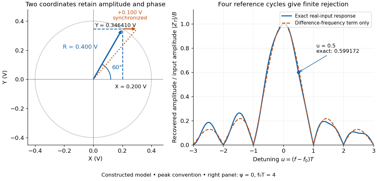

For a numerical check, use , , and an unwanted frequency . Then and the exact expression giveswhereas the difference-frequency term alone gives . An interference amplitude therefore contributes to in this constructed example. A nearby frequency can survive strongly even though the three-times-frequency component in lock-in harmonic rejection cancels exactly.
A practical lock-in amplifier's low-pass filter weights past products differently from this rectangular observation interval. Its time constant and roll-off determine near-reference rejection and settling time; narrowing detection slows the response.[ref]
Model SR830 DSP Lock-In Amplifier manual by Stanford Research Systems. Model SR830 DSP Lock-In Amplifier manual, printed p. 3-2, “Narrow band detection”; pp. 3-11–3-12, time constants and filter roll-off
Lock-in harmonic rejection 2026-10-18
Consider this original constructed input electric potential difference, with in seconds and :The unwanted component has three times the reference frequency and more than twice the wanted peak amplitude. Nevertheless, the lock-in quadratures over are exactlyso and . This is a peak amplitude calculation, not an SR830 display prediction.
To see why the larger component vanishes, multiply by each reference:Each sinusoid has zero average value of a function over a whole reference cycle. More generally, a component with integer gives products at and , whose integrals vanish over any integer number of reference cycles. This is the orthogonality behind selecting a Fourier coefficient with sinusoidal references. A nonsinusoidal reference can contain additional frequencies and need not have the same rejection property.
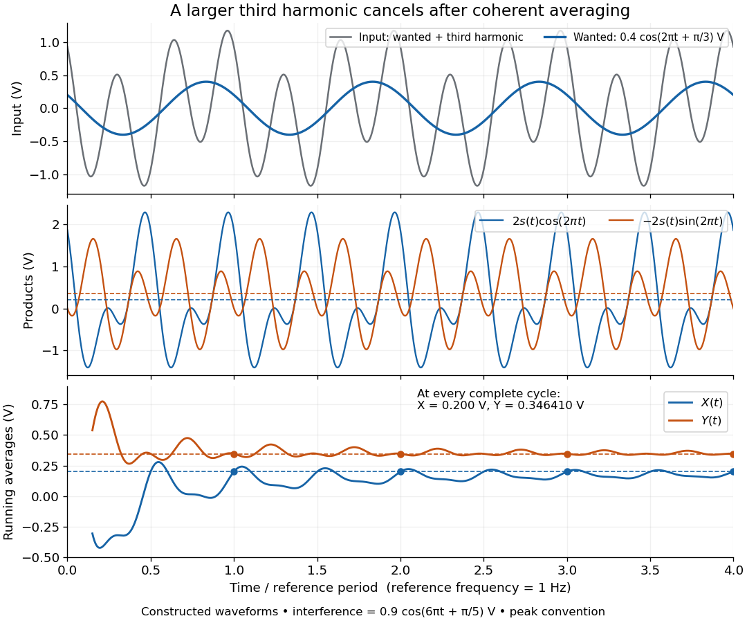

An unwanted component at the reference frequency survives. If is added to the input, its coordinate vector adds to the wanted one:For example, adding with to the wanted component gives , , , and phase difference . Longer averaging cannot separate these two synchronized contributions.
Lock-in quadratures Created 2026-10-18 Updated 2026-10-20
Let the input electric potential difference be , with peak amplitude , angular frequency , and phase difference relative to . For an observation interval containing an integer number of cycles, each lasting one period of a function, , define the lock-in quadratures in a peak convention:These integrals average the products with dimensionless references and ; and have the input's units. The minus sign makes positive give positive . The trigonometric functions giveThe oscillating terms have zero integral over the stated interval, proving and . Their orthogonality turns an oscillating signal into two constant coordinates.
Represent those coordinates as a vector, or as the complex number . Its modulus and complex argument recover the peak amplitude and phase difference:Here selects the angle with the correct signs of both coordinates, rather than applying the arctangent to and losing the quadrant. When , the amplitude is zero and the phase difference is undefined. When , despite a nonzero signal; measuring prevents this blind spot. Rotating both references by a fixed angle rotates the coordinate vector but preserves .
The factors of two above deliberately recover peak amplitude. The SR830 instead reports the selected sinusoidal component in root mean square units: in a calibrated, zero-offset display, . For this is , while the peak-to-peak span of that component is . Display normalization, reference sign, gain and angle units must be checked for the particular instrument.[ref]
Model SR830 DSP Lock-In Amplifier manual by Stanford Research Systems. Model SR830 DSP Lock-In Amplifier manual, printed p. 3-3, “RMS or Peak?” and “Degrees or Radians?”; pp. 3-13–3-14, output scaling and display offsets
Lithium reaction laboratory recoil 2026-10-18
Equal product masses imply equal kinetic energies and opposite momenta in the center of mass frame. The laboratory frame has nonzero initial momentum because the proton is moving. Conservation of momentum therefore forbids the two laboratory momenta from always being equal and opposite. The products are equal in laboratory kinetic energy only for particular emission directions, not for every event.
An exact two-body calculation makes this distinction quantitative. Write , , , and for incident kinetic energy. Express every quantity below in the same energy units; is momentum times the speed of light. For a stationary target,Here is the center-of-mass energy, and is the center-of-mass speed divided by the speed of light. Each outgoing alpha particle has center-of-mass total energy and momentum-times- magnitude . A Lorentz transformation gives the paired laboratory kinetic energies, with measured from the incident beam in the center of mass frame:Their sum is independent of and equals . Their difference is ; the symmetry belongs to the product interchange and the center of mass frame.
For the chosen model, subtract electron rest masses from each neutral-atom mass, neglect electronic binding energies, and use .[ref]
CODATA recommended values of the fundamental physical constants: 2022 by National Institute of Standards and Technology. CODATA 2022 wall chart, electron mass, energy equivalent in MeV
At , the paired laboratory kinetic energies are approximately and ; at both are approximately . In the latter case both products have a forward laboratory momentum component, so even equal laboratory kinetic energies do not imply back-to-back laboratory trajectories. A real thick target and finite detector acceptance would broaden or select these ideal kinematic possibilities. Syukuro Manabe Created 2026-10-18 Updated 2026-11-05
Syukuro Manabe and Richard T. Wetherald modelled an atmosphere relaxing toward radiative-convective equilibrium and studied its response to changes in factors including carbon dioxide. Their prescribed relative humidity lets water vapour change with temperature.[ref]
Thermal Equilibrium of the Atmosphere with a Given Distribution of Relative Humidity by Syukuro Manabe and Richard T. Wetherald. 1967 Abstract: equilibrium model and water-vapour adjustment
This couples radiative transfer with vertical thermal adjustment, making the feedback assumptions explicit. A simpler dry or fixed-water-content atmosphere need not predict the same equilibrium response.
Richard T. Wetherald Created 2026-10-18 Updated 2026-11-05
Richard T. Wetherald and Syukuro Manabe calculated atmospheric radiative-convective equilibrium with a prescribed relative humidity distribution. Allowing the water-vapour content to adjust with temperature changed the sensitivity compared with fixing absolute humidity.[ref]
Thermal Equilibrium of the Atmosphere with a Given Distribution of Relative Humidity by Syukuro Manabe and Richard T. Wetherald. 1967 Abstract: humidity assumptions and equilibrium sensitivity
The calculation demonstrates why a humidity constraint is a physical modelling assumption: it controls part of the radiative feedback as the atmosphere warms.
Gasper J. Piermarini Created 2026-10-18 Updated 2026-10-20
Director (liquid crystals) 2026-10-18
An unoriented local axis: and describe the same orientation.
There are unlisted articles, also show them or only show them.