
Quarter-wave impedance transformer 2026-10-18
A lossless intermediate section of positive real characteristic impedance matches unequal real exterior characteristic impedances when and its propagation wave phase is an odd multiple of . The length is an odd quarter of the internal wavelength. This principle also applies to the characteristic impedance of a stretched string.
For a uniform intermediate string of length , put . Continuity of displacement and transverse force gives the displacement reflection coefficientAt real positive mechanical impedances, the denominator never vanishes. Its numerator vanishes only if and . Thus unequal exterior strings require the quarter-wave condition. Equal exterior strings with a different middle string instead transmit perfectly at integer half-wavelengths; if all three mechanical impedances agree, every frequency is matched.
Maximum power transfer theorem Created 2026-10-18 Updated 2026-10-20
A Thévenin equivalent voltage source with positive source resistance supplies load power to a real resistive load. Differentiating gives its maximum at . With reactive impedances and fixed source impedance, conjugate matching maximizes the average delivered power. Maximum delivered power is distinct from maximum efficiency; at a real resistive match half of the source's internally generated power is dissipated in .
Additive identity 2026-10-18
An identity element for addition: . In a vector space, it is the zero vector; among matrices of fixed dimensions, it is the zero matrix.
Focal-distance identity for a hyperbola Created 2026-10-18 Updated 2026-10-20
For , let and place the foci of a conic at . On the right branch write , . Direct expansion givesSince , both square roots are positive and . On the reflected left branch the signed difference reverses, while its absolute value stays . This proves the constant-difference characterization of a hyperbola and keeps track of which branch a hyperbolic function parametrization covers.
For an ideal gas with constant composition, set , where is the mean particle mass. Constant downward gravitational acceleration and give by hydrostatic equilibrium. Integration gives , and the ideal gas law gives the displayed mass density ratio. The isothermal limit is .
Huber location response to one outlier 2026-10-18
Hold fixed and move only the sixth observation . For , the sample mean is , the sample median is , and the Huber location estimator with fixed stays at . Once , its Huber score is already ; moving it farther changes the Huber loss but leaves the root unchanged.
For a closer view of the transition, the exact Huber location estimator over isTo verify the first branch, when the score of is saturated and the other five scores sum with it to . When , the score of is saturated instead, giving the same expression. At , the moving observation saturates too, and the equation becomes . The piecewise formula is continuous at the transition.
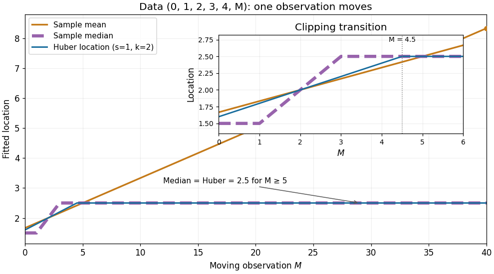

The rising sample mean comes from an unbounded linear score, the flat distant-outlier response from a bounded Huber score. This is a finite-data response curve with a specified scale and threshold, rather than a population influence function or a general claim about arbitrary numbers of outliers.
Zero-natural-length spring Created 2026-10-18 Updated 2026-10-20
An ideal spring with stiffness and zero natural length has extension equal to the distance between its endpoints. Its elastic potential energy is exactly , and its force on endpoint 2 is . Thus its Cartesian stiffness is isotropic and constant. Coupled systems of such springs have exactly linear displacement equations after a constant force, such as gravity, is absorbed into the equilibrium position. This special model differs from an ordinary finite-natural-length spring, whose transverse small-motion stiffness depends on its tension and equilibrium length.
Slope parameter for a homogeneous first-order equation Created 2026-10-18 Updated 2026-10-20
An implicit homogeneous first-order differential equation , where , can be reduced by treating the slope as an auxiliary variable. Differentiating givesWhere the divisions are valid, this is a separable differential equation. Constant slopes lost when dividing by must be checked in the original equation.
For , the reduced equation is and its nonconstant solutions obey . Substitution recovers the parabolas , together with the constant solution . Real graph branches must have , and the original restrictions , still apply. The constant slopes solve the reduced equation but are excluded from the original equation.
History of Hölder's inequality 2026-10-18
Otto Hölder's 1889 paper begins with a weighted-mean inequality for a function with increasing derivative. In current terminology, its opening statement is a weighted form of Jensen's inequality: applying a convex function after taking a weighted mean gives a lower bound for the weighted mean of its values. This connects product estimates to the geometry of convex functions, rather than treating them as isolated formulas.[ref]
Ueber einen Mittelwerthssatz by Otto Hölder. Otto Hölder, Ueber einen Mittelwerthssatz (1889), §§1–2, printed pp. 38–39: weighted means and increasing derivative
Probabilistic use of Hölder's inequality 2026-10-18
On a probability space, the same inequality readsIf the displayed moments are finite, the product is an integrable random variable. The random variables can be dependent: the estimate controls their possible overlap without assuming a factorization of the expected value. This is useful when a calculation needs the product to be integrable but the joint probability distribution is complicated.
Equality in Hölder's inequality 2026-10-18
For and nonzero factors in their respective Lp spaces, equality in the product-integral bound holds precisely whenIn other words, the normalized powers match. Zero factors give the trivial equality separately. For real vectors, equality for the signed finite sum also needs the nonzero coordinate products to have a common sign; otherwise the preceding triangle inequality loses information.
For and on , with , ,Changing only to gives , and both sides become . The factors need not be equal: their conjugate powers are what must agree after normalization.
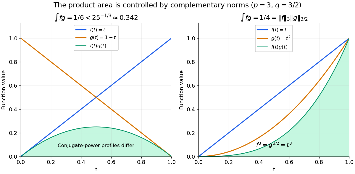

The proof outline makes the equality condition natural. Normalize and . The Young inequality gives ; integration yields . Equality requires almost everywhere. The endpoint proof uses the essential supremum directly, so it does not need division by at .
Finite-vector example of Hölder's inequality 2026-10-18
Take , , and vectors and . Their coordinate products are , soTheir Lp norms give the larger boundThus cancellation explains , and Hölder's inequality explains the remaining gap between and the norm product. Small signed sums need not imply small individual coordinate products.
Now keep and choose . The coordinate products are , with no cancellation, andThe matching powers are , namely .
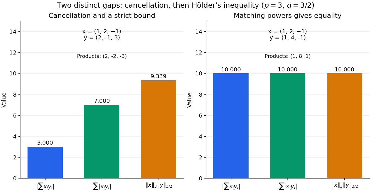
Cancellation and Hölder's inequality account for two different gaps
. Two original finite-vector calculations with , . The first pair has signed sum , absolute-product sum and norm-product bound approximately . The second pair attains equality at . The diagrams show calculated values, with no simulated data. Details.
Conjugate exponent 2026-10-18
The conjugate exponent of is , so . The endpoint conventions pair with and with . Examples are , and . The exponents themselves need not add to one; their reciprocals do.
Hohmann transfer time 2026-10-18
A Hohmann transfer orbit between coplanar circular Kepler orbits of radii traverses half an elliptic orbit of semi-major axis . Kepler's third law therefore gives . Relative to the initial orbital period , . Radii must be measured from the attracting centre, rather than from its surface.
Hohmann transfer impulse fractions Created 2026-10-18 Updated 2026-10-20
For a Hohmann transfer orbit from radius to , with and initial circular speed , conservation of orbital energy and angular momentum gives transfer endpoint speeds and . The required prograde impulses areIf the spacecraft mass is constant and fuel use is proportional to impulse magnitude, these also give the fuel fractions relative to a budget with total speed change . Their sum is a sum of magnitudes, even though the burns occur at different positions and directions.
Three-step model of high harmonic generation Created 2026-10-18 Updated 2026-10-20
For an original classical calculation of the return step, neglect the residual ion's Coulomb force after release. Take a spatially uniform driving electric field , an electron of electric charge and mass , and zero initial position and velocity at . With and , integrating Newton's second law givesA return requires and . Define the cycle-averaged free-electron quiver kinetic energySearching the first-return solutions for release phases gives a maximum near and , with . For a chosen ionization energy , recombination into the initial state can therefore emit a photon with energy up to approximately in this model. This is an upper return-energy scale, not a prediction of the emitted yield. It omits release probabilities, quantum interference, propagation, phase matching and depletion of the neutral gas.
The calculation explains why a long driving wavelength can increase the available return energy: at fixed , grows as . It does not say that conversion efficiency improves. The electron must return with a probability amplitude for emission that survives the microscopic dynamics and adds coherently across the gas.
Hermite polynomial derivative recurrence Created 2026-10-18 Updated 2026-10-31
For the physicists' Hermite polynomials , the displayed recurrence holds for , while separately. Put . Differentiating exactly times using the Leibniz rule yieldsDifferentiating the defining product for then givesThe nonnegative integer convention is essential for the derivative-based definition; no negative-order derivative or is needed.
Hénon-Heiles potential 2026-10-18
The potential energy in the Hénon-Heiles system has the following expression in polar coordinates:so it is invariant under rotation through . Solving gives a strict local minimum at the origin and three saddle points, at and . All three saddle points have value . Their common level set factors exactly:Thus this level set is the union of the three lines and . They bound an equilateral triangle containing the local minimum. The Hessian matrix is the identity at the origin; at each of the other three stationary points it has eigenvalues and . For energies , the central accessible region is bounded; above that value the three saddle passages allow paths from the centre to arbitrarily large radius. This follows directly from the radial potential: in each direction with , its radial maximum occurs at , with value .
Maximum-volume cuboid in a hemisphere 2026-10-18
For a closed hemisphere of radius , take a rectangular parallelepiped with a face on the flat base, base half-widths and height . Its curved-boundary constraint is and its volume is . A Lagrange multiplier gives , yielding the displayed maximum. The full edge lengths are .
This bound remains valid when arbitrary orientations are allowed. Write a cuboid's half-edge lengths as , its center components in its orthonormal edge basis as , and the vertical unit-vector components as . Containment above the base plane requires . Hence for at least one : otherwise every contributing term would be strictly smaller than its required bound. Its farthest vertex has squared distanceContainment in the sphere bounds the right side by . The arithmetic-geometric mean inequality then gives , so the full volume cannot exceed the displayed value. The constructed cuboid attains it. With strict containment and no boundary contact, the same value is a supremum.
Use the coordinate conventionIn this convention the Heisenberg group over a prime field has the productThe subset is an Abelian subgroup of order : the middle coordinate in a product is , which is symmetric in the factors. Also lies in . The map is a surjective group homomorphism to the additive group of , with kernel of a group homomorphism . Hence is a normal subgroup of subgroup index , and its left cosets are exactly the level sets of .
For odd , an explicit group isomorphism from to the additive group isThe term in matrix multiplication cancels the cross term in . Thus is an elementary abelian group, isomorphic to .
There are unlisted articles, also show them or only show them.