
Bubble-chamber track Created 2026-10-18 Updated 2026-11-05
A bubble-chamber track is a line of growing vapor bubbles seeded by ionization along a charged particle path in a superheated liquid. The bubbles scatter illumination and can be photographed from multiple directions to reconstruct the path in three dimensions.
In a known magnetic field, curvature constrains the particle's momentum and the sign of its electric charge; increasing ionization toward a stopping point can add information about energy loss. Bubble size and photographic blur set the visible trail width, so that width is not the particle's physical diameter. Neutral particles can remain invisible until an interaction produces charged secondaries.
Work by Bruno Pontecorvo 2026-10-18
Work by Bruno Benedetto Rossi Created 2026-10-18 Updated 2026-10-24
Work by Bruce Elsmore 2026-10-18
Work by Brian Schmidt 2026-10-18
Work by Brian D. Josephson Created 2026-10-18 Updated 2026-10-24
For an entire function , let with noninteger real , and choose the branch of the complex logarithm with . On the cut ray , the bank whose argument approaches has value , while the other bank has argument approaching and value . The signed jump is therefore when defined as . Stating the branch and order of subtraction removes the sign ambiguity. A keyhole contour uses this phase relation to convert its two bank integrals into a constant multiple of one real or radial integral.
Bound charge Created 2026-10-18 Updated 2026-11-05
The effective electric charge associated with electric polarization is bound charge. For polarization density , its volume charge density is . At a boundary with unpolarized surroundings, its surface charge density is , where is the outward unit normal vector.
Delta-shell Born amplitude 2026-10-18
For a real shell potential , define and , with value one at zero. Angular integration of its three-dimensional Fourier transform gives , where the momentum transfer has wave-number magnitude . Substitution in the first Born approximation proves the displayed scattering amplitude. It is real. Its squared modulus is a nonzero order- differential scattering cross-section, whose optical theorem counterpart requires the order- imaginary part of the forward amplitude from the next Born term. Thus squaring the first-order amplitude does not supply a consistently unitary second-order amplitude.
Born amplitude for a Yukawa potential Created 2026-10-18 Updated 2026-10-24
For , with real and , the first Born approximation gives the scattering amplitudeIndeed, orienting the polar axis along the momentum transfer gives the angular integral , and the remaining integral is . The differential scattering cross-section is .
The limit at fixed nonzero produces the Rutherford differential cross-section for a Coulomb potential. The unscreened interaction has long range, so this limiting calculation by itself does not establish the validity of a naive Born approximation to the full Rutherford scattering state. The exact Rutherford scattering amplitude has an additional phase, while its modulus agrees with the Rutherford differential cross-section.
Discharge spectra and the Bohr model Created 2026-10-18 Updated 2026-10-20
In On the Constitution of Atoms and Molecules, Part I (1913), pp. 8–9, Niels Bohr interprets existing hydrogen discharge and astronomical spectra. Electrical discharge in a vacuum tube removes electrons; recombination supplies spectral lines. This is a theoretical interpretation, without a reported spectrograph of his own.[ref]
On the Constitution of Atoms and Molecules, Part I by Niels Bohr. Part I, section 2, pp. 8–9: existing spectra
An actual optical obstacle appears in Theodore Lyman's measurements: hydrogen discharge light entered an evacuated spectrograph directly through a slit, avoiding a transmitting window. A concave reflection diffraction grating dispersed the light onto photographic film. Pumping preserved the vacuum; a second slit supplied a known spectral displacement for wavelength calibration. Gas contamination and vacuum leaks limited the measurement. This apparatus resolved ultraviolet spectral lines; it did not image orbits.[ref]
Theodore Lyman, Pioneer of Ultraviolet Vacuum Spectroscopy by Paul Horowitz. Paul Horowitz, Theodore Lyman, Pioneer of Ultraviolet Vacuum Spectroscopy, pp. 3–4, figures 2–5: windowless discharge connection, grating, film, pumping and dual-slit calibration
For a separate original calibration exercise, suppose an idealized spectrograph returns synthetic vacuum line positions for , with chosen additive offset . Assume its dispersion scale is already known and only this offset is uncertain. Compare the finite-mass prediction with the fixed-nucleus prediction . Calibrate each model using only the line: . Then hold that offset fixed and test the other lines with residualsFor the finite-mass model every . The fixed-nucleus model has and residuals , , . Algebraically : one additive calibration cannot absorb a multiplicative change of the wavelengths. Allowing an unknown multiplicative dispersion factor as well would make the two models degenerate in this exercise, so independent scale calibration matters.
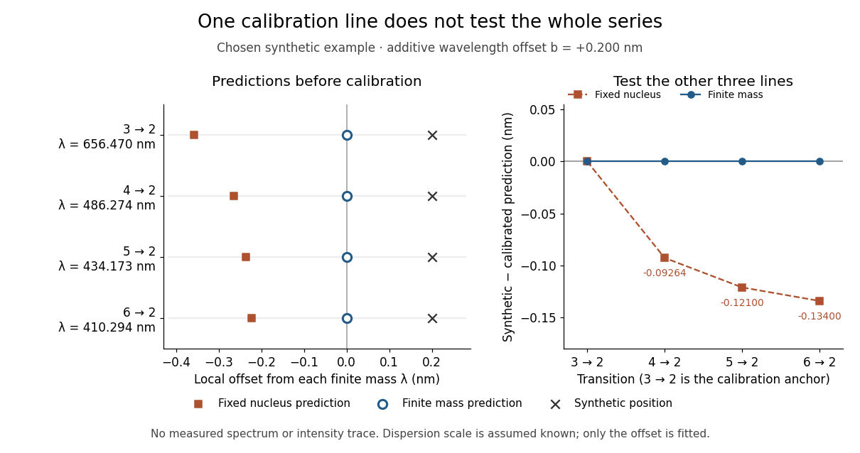
Balmer series predictions tested after calibrating one line
. Original synthetic calibration exercise with chosen . Left: finite-mass vacuum predictions and deliberately offset synthetic positions, displayed on a separate local wavelength axis for each line. Right: model residuals after anchoring the line; the remaining three lines test the prediction. Symbols are exact synthetic inputs and calculated results, not historical observations, error bars or an intensity trace. Details.
Hydrogen transition wavelengths in the Bohr model Created 2026-10-18 Updated 2026-10-20
For emission take integers . Applying conservation of energy to the model's internal energy difference, while neglecting the much smaller whole-atom photon recoil, givesThus Johannes Robert Rydberg's Rydberg formula is a difference of two energy levels expressed as a spectroscopic wavenumber. The same constants determine every line; there is no new parameter for each electronic transition. With the chosen inputs, . All wavelengths below are calculated in vacuum, not air, and are rounded model predictions rather than historical measurements.
The conventional names commemorate Theodore Lyman and Johann Jakob Balmer. Fixing produces the ultraviolet Lyman series, beginning with the Lyman-alpha line; fixing produces the Balmer series. As , the wavelength approaches : at the Lyman limit and for the Balmer series. Crowding follows directly from . Discreteness therefore coexists with a series limit.
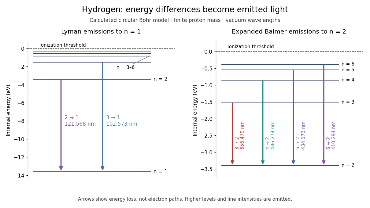

Correct line positions do not give wave intensities, lifetimes or electric-dipole selection rules for hydrogen. Those require a theory of the wavefunctions and their coupling to electromagnetic radiation. The circular model also omits spin, relativistic corrections and the Lamb shift. Its successful gross energy levels do not make its assumed orbits modern atomic orbitals.
Circular-orbit derivation of the Bohr model Created 2026-10-18 Updated 2026-10-20
Consider a single electron of mass and a point atomic nucleus of mass and positive electric charge , with the elementary charge. Use nonrelativistic classical mechanics, omit external fields and interactions with other electrons, and writeHere is the Coulomb two-body reduced mass, the vacuum permittivity, and the Planck constant. The separation and relative speed describe the two-particle relative coordinate; neither body is silently pinned in place. The electron's own radius about the centre of mass is .
For the assumed circular orbit, Coulomb's law provides the required centripetal acceleration, and the imposed orbital angular momentum condition isSubstitute into the first equation and cancel to obtainThe kinetic energy is and the Coulomb potential energy is , with zero energy at infinite separation. HenceThis derives the energy sequence from the stated circular model; the modern Schrödinger equation derivation is the distinct series-termination quantization of the Coulomb radial equation. The radius above scales as , whereas the binding energy scales as . The Bohr radius article supplies the corresponding Coulomb potential length scale. The nonrelativistic assumption requires , with the speed of light.
For an original numerical example choose , , , , , , and . Treat these as stipulated constants for the calculation. They give , , and , where denotes an electronvolt. At , and ; the ground-state ionization energy is .
Taking gives . A finite nuclear mass reduces every binding energy by and increases each separation by . This follows from relative motion, not a fitted correction to individual spectral lines. Replacing the atomic nucleus by a heavier isotope changes the same factor, providing another check of the model.
Bloch Hamiltonian Created 2026-10-18 Updated 2026-11-05
The Bloch Hamiltonian acts on the cell-periodic part of a Bloch state at fixed wavevector. If , defineFor a scalar periodic potential, its kinetic term is on cell-periodic functions.
Solving this family of cell problems produces electronic band structure. In a tight-binding description, the Bloch Hamiltonian is a matrix on the orbitals within a primitive cell, not the full infinite real-space matrix. Basis choices can change its entries without changing the physical band energies. The distinction between the full wavefunction and its periodic factor also matters when computing matrix elements and geometric phases.
Inversion symmetry 2026-10-18
Invariance under spatial inversion about a specified origin.
State counting in a Bloch band 2026-10-18
A crystal with primitive unit cells has distinct wavevectors in one Brillouin zone. For a rectangular periodic sample, , and the product of the numbers of allowed values along the three directions equals the number of cells. Each orbital-derived energy band therefore holds states per spin orientation, or with twofold spin degeneracy. This means two states per primitive cell per spin-degenerate band, independently of how many atoms the cell contains.
Shockley junction transistor proposal 2026-10-18
William Shockley's proposal used transport through the bulk of a semiconductor, rather than coupling between two surface points. The base must be thin enough for injected minority carriers to reach the collector. Two separately wired diodes do not supply that shared transport region. The proposal was a design principle; producing a working device required further control of material properties.[ref]
Transistor technology evokes new physics by William Shockley. Printed pp. 368–370
Magnetic field of a finite straight wire 2026-10-18
Take a wire segment on the axis, with source positions for , and positive electric current along . Observe at , where is the perpendicular distance to the wire's supporting line. Choose rightward and upward, so points out of the page. ThenThus the magnetic field points into the page by the right-hand rule. The Biot-Savart law and an elementary antiderivative giveFor an original worked example, choose , , , and . Use for these rounded calculations. Each endpoint contributes , soThese are calculated inputs and output, not laboratory data. The two endpoint angles measured from the perpendicular each have sine ; this recovers the equivalent endpoint-angle formula without depending on a diagram's angle-sign convention.
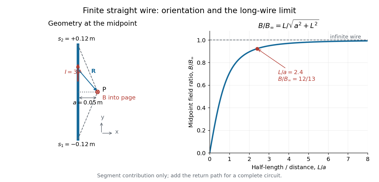

For a segment centered on the perpendicular foot, , . Its magnetic field magnitude isThe limit gives , consistent with Ampère's circuital law for an infinite straight wire. In the example, and : the infinite-wire value overestimates the segment value by , or about of the segment value. For , the isolated segment contribution instead behaves as . The complete localized electrical circuit has a different far-field behavior: return-path contributions cancel this leading segment term, leaving a magnetic dipole field when its magnetic dipole moment is nonzero. Segment and whole-circuit limits must be distinguished.
The SI units check directly: has units , the tesla. The apparent divergence as is a failure of the thin-wire model near the conductor, not a prediction of infinite magnetic field inside a real wire. This calculation gives only this segment's contribution; include the return wires before comparing with an apparatus.
Current element Created 2026-10-18 Updated 2026-10-20
A current element is the oriented infinitesimal wire contribution inside the Biot-Savart law. For uniform axial current density across wire cross-sectional area , and imply . This reduces a volume integral to a line integral in the thin-wire approximation. It is an integration contribution, not an isolated steady source. Conventional current runs opposite the drift of negatively charged electrons.
Magnetic-field cancellation of an arc and tangent leads Created 2026-10-18 Updated 2026-10-20
For a circular arc of radius carrying clockwise electric current and subtending angle , with two tangent semi-infinite leads extending on the crossing side of the arc, the axial magnetic field at height above the centre isThe crossing is insulated. The positive term is from the two leads and the negative term from the arc, with out of the clockwise-current plane. The Biot-Savart law yields the lead integral . Cancellation of the axial component gives the title formula, expanding to in radians. This is cancellation of one component away from the plane, not necessarily the entire magnetic field.
There are unlisted articles, also show them or only show them.