
Past exam of the mathematics course of the University of Cambridge 2006 iii Paper 54 4 Solution Created 2026-10-03 Updated 2026-10-14
First complexify the Clifford algebra in spacetime dimensions. Multiplying appropriate generators by converts the signature to the Euclidean form without changing the complex module dimension. Pair the generators intoThe Clifford algebra relations giveThe commuting occupation operators have eigenvalues zero or one. Choose a nonzero state killed by every ; repeated annihilation reaches such a state in any finite irreducible module. Acting with distinct creation operators produces the occupation statesTheir distinct occupation patterns make them linearly independent, and their span is invariant under every Clifford generator. Irreducibility therefore makes it the entire Dirac module. This derives the even-dimensional Clifford spinor dimension:The chirality matrix is a phase-adjusted product of all generators. It squares to one, anticommutes with each generator and acts as occupation parity up to an overall sign. Its two eigenspaces each have states. The even Clifford algebra, and hence the connected spin group, preserves them, giving irreducible Weyl spinors of complex dimension . A Majorana spinor imposes a reality condition only in signatures where it exists; simultaneous Majorana and Weyl conditions are not available in every even dimension.
In Lorentzian ten dimensions, the complex Dirac module has dimension , and a Weyl module dimension . A Majorana-Weyl spinor is allowed and has real components before its equation of motion. The massless Dirac equation leaves eight physical gaugino polarizations. A ten-dimensional massless gauge field also has physical polarizations. Thus ten-dimensional super Yang-Mills theory has eight bosonic and eight fermionic states per gauge generator, with sixteen real supercharges.
For dimensional reduction, take a flat six-torus with periodic fermions and retain fields independent of its coordinates. Split into and six internal components , . The latter are four-dimensional real adjoint scalar fields. Under the spin groups of the two factors, a ten-dimensional chiral spinor decomposes asfor , with . The Majorana condition relates these conjugate pieces, leaving four independent four-dimensional Weyl spinors. The supersymmetry parameters reduce in exactly the same fashion: sixteen real charges are four four-dimensional supersymmetries. The resulting field content isThe on-shell counts are bosonic and fermionic states, as required. The internal spin group supplies the R-symmetry of the reduced action.
To derive its scalar potential, use Hermitian gauge matrices and a positive trace inner product, withIf the internal volume is , integration gives . Since internal derivatives vanish,With mostly-minus spacetime signature, has an extra minus sign and the double sum over mixed indices gives a factor two. Rescale and to canonical fields. The resulting bosonic Lagrangian iswhere . A commutator of Hermitian matrices is anti-Hermitian, so the last term is minus a nonnegative scalar potential:The sum is over ordered internal pairs; a sum over would instead have coefficient . Trace normalization merely changes the matched gauge-coupling convention.
The origin attains zero potential, so the global minima are exactlyFor a compact connected gauge group, a commuting tuple is simultaneously conjugate into a Cartan subalgebra. Write , where is the rank. Every choice of the real numbers has zero potential. After the residual Weyl group identifications, the classical commuting-scalar vacua of four-dimensional N=4 Yang-Mills theory form in the four-dimensional theory. For one may describe them as six simultaneous diagonal matrices, with tracelessness and permutations of their common eigenvalue labels. Varying these eigenvalues changes gauge-invariant configurations while leaving , proving the existence of genuine flat directions of a scalar potential, not just gauge-equivalent directions. Generic values break the gauge group to its maximal torus; coincident eigenvalue vectors produce enhanced unbroken gauge symmetry. If one keeps a finite compact torus rather than the four-dimensional limit, large gauge transformations add periodic identifications of the Wilson-line coordinates.
Past exam of the mathematics course of the University of Cambridge 2006 iii Paper 54 3 Solution Created 2026-10-03 Updated 2026-10-14
At the usual two-derivative order, the two-derivative global supersymmetric gauge action isHere is the chiral field-strength superfield, distinguished from the superpotential . The Kähler potential is a real gauge-invariant function, defined up to a Kähler transformation; supplies the scalar kinetic metric. The superpotential is a gauge-invariant holomorphic function of the chiral superfields. The symmetric gauge kinetic function is holomorphic and transforms so that its contraction with the field strengths is gauge invariant. Its real part supplies the gauge and gaugino kinetic coefficients and must be positive on physical configurations; its imaginary part supplies the topological angle. The final constants are Fayet–Iliopoulos terms, normalized so that they contribute when has highest component .
For the simple non-Abelian gauge group specified in the question, . Invariance of a proposed requires . A simple Lie algebra equals its commutator algebra, so no nonzero invariant covector exists. This proves that Fayet–Iliopoulos terms require an Abelian gauge factor. The last term above describes the customary Abelian extension, not an additional arbitrary coupling of the simple group.
For a renormalizable theory, after choosing matter bases the functions reduce toOnly gauge-invariant monomials are included. A nonconstant would produce interactions of dimension greater than four. Here the gauge coupling is absorbed into the connection in , while in the holomorphic normalization. A constant has no dynamical effect in global supersymmetry. The original arbitrary functions remain useful for a nonrenormalizable two-derivative effective theory, but the following argument restricts to the requested renormalizable setting.
To analyze perturbative corrections, use a local Wilsonian effective action with a nonzero infrared cutoff and keep the same elementary fields. Introduce nondynamical background chiral superfields into its F-term part:One may additionally promote each polynomial coefficient to its own chiral spurion to track flavor charges. Treating the couplings as fields ensures that a local chiral integral depends holomorphically on : antichiral dependence would violate the chirality constraint unless accompanied by derivatives or rewritten as a D-term. This is the key use of holomorphy, rather than an assumption that all effective-action terms are holomorphic.
Give R-charge one, the matter fields charge zero, charge two and charge zero. Then the chiral measure has charge minus two, has charge two, and has charge one. These assignments define formal spurionic symmetries even if fixed numerical couplings do not enjoy the corresponding physical symmetry. An anomalous transformation is accompanied by the appropriate shift of the gauge-coupling spurion; nonperturbative dependence can record that anomaly.
For the superpotential non-renormalization argument, perturbation theory is insensitive to continuous shifts of the topological angle, which shifts the imaginary part of . A holomorphic coefficient invariant under every such shift is independent of by the Cauchy-Riemann equations. This proves perturbative gauge-coupling independence of the Wilsonian superpotential. At fixed infrared cutoff the perturbative expansion is regular near zero superpotential couplings. R-charge two therefore forces an allowed correction to be linear in , rather than involving , or inverse powers of . Flavor charges impose the corresponding monomial selection rules.
The remaining coefficient can be evaluated at zero gauge coupling. Free chiral propagators join a chiral and an antichiral endpoint. A single holomorphic superpotential vertex cannot close a loop; adding antichiral vertices violates holomorphy, while adding holomorphic vertices violates the linear spurion degree. Consequently the coefficient is its tree value. This proves, rather than merely quotes, the perturbative resultThe fixed-cutoff regularity matters: integrating out a whole massive multiplet can introduce inverse masses at tree level, and infrared-singular one-particle-irreducible expressions are not this local Wilsonian superpotential.
For the gauge kinetic function, R-charge zero excludes regular positive powers of in its perturbative coefficient. Flavor spurions cannot repair this without forbidden antichiral or singular dependence. A topological-angle shift changes the tree gauge term only by its topological contribution, so the correction is invariant under the shift. Holomorphy then makes it independent of . An -loop correction to the inverse gauge coupling carries the weak-coupling behavior : only one loop has the required coupling-independent behavior. Hence the one-loop exactness of the holomorphic gauge kinetic function givesup to a one-loop matching constant. The coefficient follows from the usual one-loop field contributions: gauge bosons and an adjoint Weyl gaugino contribute , while a chiral Weyl fermion and complex scalar contribute . Holomorphic logarithmic thresholds appear when massive fields are eliminated. This statement is about the holomorphic Wilsonian coupling, not a canonically normalized physical gauge coupling, whose running need not be one-loop exact.
The Kähler potential is integrated over all of superspace. It can depend on , on both and , and on both matter chiralities. These neutral combinations allow ordinary loop corrections, such as a Yukawa-dependent correction to , and no analogous argument forbids higher loops. ThusIts wave-function renormalization changes physical superpotential couplings after canonical normalization even though holomorphic vertex coefficients do not change. For a single field with kinetic coefficient , for instance, and .
Finally consider perturbative renormalization of a Fayet–Iliopoulos term in an Abelian extension. A term must be invariant under for arbitrary chiral . Projection of the variation requires . An arbitrary algebraic function of background chiral spurions and their conjugates fails this requirement unless it is constant. Therefore a general coupling-dependent local FI counterterm is forbidden. The one-loop tadpole from charged scalars can still giveIt is independent of interaction couplings in the connection normalization used above and proportional to the trace of the Abelian charge generator. Higher-loop diagrams require interactions and cannot produce the permitted coupling-independent additive term. Thus a traceless Abelian charge generator has no additive perturbative FI renormalization in this exactly supersymmetric setting; otherwise a one-loop, regulator-dependent tadpole is possible. Vector-field normalization can change the reported canonical parameter, and soft breaking falls outside this proof. For the specified simple group, gauge invariance forbids before and after corrections.
These are perturbative statements. Instantons or other nonperturbative effects may produce symmetry-allowed holomorphic terms, for example dependence on , so neither the superpotential result nor the one-loop gauge result should be misread as forbidding all nonperturbative corrections.
Past exam of the mathematics course of the University of Cambridge 2006 iii Paper 54 2 i Created 2026-10-03 Updated 2026-10-14
Past exam of the mathematics course of the University of Cambridge 2006 iii Paper 53 4 Solution Created 2026-10-03 Updated 2026-10-14
Use and keep each constant odd supersymmetry parameter on the left. The transformation of a fermion may be written or , since the bosonic derivative commutes with the parameter. The variation itself is even, so it obeys the ordinary product rule; the signs below arise when moving an odd parameter past an odd field.
First consider the transformation. Suppress target indices and put . Its bosonic part varies asFor the first fermion, moving to the left givesThe second fermion does not vary under . Since , these terms combine to . The other parameter gives the same cancellation with and . ThereforeThis proves worldsheet supersymmetry invariance up to the rigid worldsheet supersymmetry boundary term, without using field equations.
For an open string, the boundary term is part of the invariance statement. For example, a Neumann endpoint has and compatible fermion gluing , . The spatial boundary flux vanishes when . Both endpoints must admit the same preserved parameter. Opposite gluing signs, giving the Neveu–Schwarz sector, do not preserve a nonzero constant parameter at both ends. Thus the local bulk identity and the existence of a global rigid charge on a particular open-string sector are distinct. The local superconformal symmetry remains the basis of the string constraints; this is consistent with the spin-structure obstruction to constant worldsheet supersymmetry.
Now write and , . The other two components vanish. The action implies , and , so these supercurrents are chiral and conserved locally. At equal time, the given canonical commutation relations implyWith , contraction with this commutator givesThe parameter-weighted charge is even. Since the parameters anticommute with the fermions,Using the PDF's normalization yieldsThus the charge generates all the specified supersymmetry transformations. Dropping the factor in the fermion anticommutator, as happens in the converted TeX, would fail this check. The original PDF has the correct factor.
To calculate the supercurrent bracket, put and . The equal-time bosonic relations giveBosonic and fermionic fields commute. Expanding the two current products, commuting the bosonic factors once and using the fermion anticommutator gives the noncentral partFor an ordinary smooth bilocal coefficient, the distributional derivative identity isFor the fermion bilinear, its coincident classical value, or its coincident normal-ordered value, is zero by antisymmetry against the symmetric target metric. The second term is . Since , we have . It follows that the noncentral current bracket isThis is the canonical supercurrent bracket of free RNS matter. The other chirality similarly gives and on shell.
The printed current identity is the classical, or noncentral, part of the algebra. Fully quantized coincident products require normal ordering; the matter algebra then also has a central contact term proportional to in the current anticommutator. The 10 bosons and 10 real fermions contribute matter central charge . The central term cannot be discarded in a literal quantum operator identity, although it is irrelevant to identifying the local noncentral stress tensor above.
The other brackets close on these same currents. The stress-tensor commutator contains and and, quantum mechanically, a central term. The stress-tensor–supercurrent commutator contains and , expressing the conformal weight of . The supercurrent anticommutator contains and its central term. In a conventional normalization of Fourier modes these form the N=1 super-Virasoro algebra:Here and are central terms supported at zero total mode number; their detailed coefficients are not needed for this request. The indices are half-integers in the Neveu–Schwarz sector and integers in the Ramond sector. Opposite chiralities commute or anticommute as appropriate.
For the closed RNS string, impose a copy of the constraints in each chirality. In the Neveu–Schwarz sector, the physical conditions areIn the Ramond sector, use vacuum-normal-ordered generators with zero Ramond intercept. ThenThe Ramond zero-mode equation is essential: its square gives the mass-shell condition in this convention, , and on the oscillator ground sector it is the spacetime Dirac constraint. In a convention whose unshifted plane generator has , the zero-mode equation instead sets that shifted combination to zero; these are the same condition, not competing intercepts.
For either choice, the corresponding tilded constraints hold on the other side. Both chiral mass-shell conditions and closed-string level matching are required:The state sectors are NS–NS, NS–R, R–NS and R–R. Quotienting physical null states removes unphysical longitudinal polarizations; equivalently, use the appropriate BRST cohomology including the superconformal ghosts. A consistent superstring also specifies the GSO projection. It is an additional sector selection, not a replacement for these local super-Virasoro constraints. Physical states satisfy both chiral positive-mode and zero-mode constraints, level matching, and the null-state quotient; Ramond states additionally obey the fermionic zero-mode constraint.
Past exam of the mathematics course of the University of Cambridge 2006 iii Paper 53 3 Solution Created 2026-10-03 Updated 2026-10-14
The Polyakov action is invariant under worldsheet diffeomorphisms and Weyl transformations, . A two-dimensional metric has three local components: two coordinate transformations and one Weyl function remove these locally. In conformal gauge the factor is independent of the conformal scale, and on a flat coordinate patch the matter action isThus it is the action of free scalar fields, with their target-space contractions using the Minkowski metric. On a Euclidean sphere there are no unpunctured conformal moduli: a metric can be put into the conformal class of the round metric, and in stereographic patches the scalar action has this free-field form. This does not mean that the sphere has a globally flat metric. A spherical worldsheet here is understood after Wick rotation; it has no nonsingular global Lorentzian metric. The residual Möbius transformations and their zero modes still have to be divided out or fixed by vertex positions.
To derive the worldsheet ghost action, consider an infinitesimal diffeomorphism generated by and a Weyl variation . The metric variation separates asIntegration over the Weyl parameter removes the trace gauge condition. The trace-free part produces the Faddeev-Popov determinant of an operator mapping vectors to symmetric traceless tensors. This is trace elimination in string Faddeev-Popov gauge fixing. The stated Grassmann Gaussian integral exponentiates this determinant with an odd vector and an odd symmetric trace-free antighost .
The normalization of the operator and antighost can be chosen to match the printed convention. For example, in a flat patch take . It differs from the orbit operator only by a field-independent determinant factor. Tracelessness and symmetry give . Integration by parts, followed by exchanging two odd factors, gives . Consequently the determinant exponent is withOverall constant normalization does not affect the determinant's dependence on the fields. The Faddeev-Popov ghost fields are vectors, while the antighost fields are symmetric trace-free tensors; they are not extra target-space string excitations.
Now use , and . In these coordinates and . Tracelessness implies , so directlyThereforeFor a Cartesian check, and , reproduce the same result.
The original PDF repeats for its final ghost transformation. The second occurrence must be ; otherwise the displayed rules give two incompatible transformations for one ghost and none for the other. Write the corrected transformation as , with on the left. Then the odd left-acting BRST differential satisfies the graded Leibniz rule . Its local rules areThe last two expressions are with the matter-plus-ghost worldsheet stress tensor in the question.
Here is an off-shell check of the action variation, including the Grassmann signs. Temporarily set , , , , and . Apart from the common factor , the total Lagrangian is . Its matter variation isThe matter terms in and give the ghost-action contribution . Combining these terms with the last two matter terms produces .
The remaining contribution from the sector iswhere subscripts denote derivatives. In the last equality the terms and cancel by anticommutation. The sector has the same identity with . ThuswhereHence the total action is BRST invariant up to a boundary term, which vanishes on a closed worldsheet or under the usual compatible boundary and time-end conditions. This calculation requires no equations of motion.
Nilpotence needs a qualification for these particular chiral rules. For either ghost, , because . Thus algebraically. For the embedding, however, the graded calculation givesMixed second derivatives of cancel because . The remaining terms vanish on the ghost equations of motion, , which follow by varying the antighosts in the chiral ghost action. They need not vanish off shell. An explicit counterexample uses independent Grassmann variables : take , and one coordinate . Then .
For the antighosts, use the permitted stress-tensor identity on the classical solution space. Then . Indeed direct variation of the displayed stress tensors giveswhich vanish using the ghost equations and the free matter wave equation. Therefore two successive BRST transformations annihilate every field on shell. This is chiral conformal-gauge BRST nilpotence is on shell, not an unrestricted off-shell identity for arbitrary ghosts. Quantum BRST nilpotence additionally requires cancellation of the worldsheet anomaly, giving in the critical bosonic theory.
Past exam of the mathematics course of the University of Cambridge 2006 iii Paper 53 2 Solution Created 2026-10-03 Updated 2026-10-14
Distinguish target-space light-cone coordinates from the worldsheet labels. In target space take , so the Minkowski metric is . After conformal gauge has been chosen, the residual transformations of and may be used, on a patch with , to makeFor an open string on , the conventional normalization is . For the closed-string convention of the preceding solution, . In either case, the two Virasoro constraints readSince , they determine the longitudinal coordinate:Its oscillator content is fixed by the transverse coordinates, leaving independent fields. This is the light-cone gauge in string theory; it solves the constraints rather than imposing them afresh on each transverse state.
For Neumann boundary conditions at both endpoints, the open-string expansion isThe transverse string oscillators satisfy , , and . Define and . The solved longitudinal modes, including the zero-mode constraint, areThe critical bosonic string theory has 24 transverse bosons. Their regulated oscillator vacuum energy is , since the finite term of is . Thus the normal-ordering constant of a string is . A normalized transverse Fock space basis for general excited physical string states iswith finitely many nonzero occupation numbers. Arbitrary physical states are superpositions of this basis, with each momentum on its corresponding mass shell. The string level operator and open bosonic string mass spectrum giveAll spatial directions have free endpoints, so this string ends on a space-filling D25-brane. More generally, a D-brane has Neumann boundary conditions along its worldvolume and Dirichlet boundary conditions in its transverse directions; a D-brane has spatial worldvolume directions. A stack may additionally supply Chan-Paton factors, without changing the oscillator construction above.
To see T-duality of D-brane boundary conditions directly, decompose the compact coordinate as and define its dual by . Differentiation givesTherefore the original Neumann boundary condition becomes at each endpoint. The dual endpoint coordinate is time-independent: the dual condition is Dirichlet. Conversely a fixed endpoint in becomes Neumann in the dual coordinate. For a circle, the T-duality radius is . A wrapped Neumann brane loses one spatial dimension in the dual picture, for example D25 becomes D24. The two dual endpoint constants need not be identical; their positions encode the original Wilson-line data.
For the separated-brane problem, use two static parallel D-branes and no relative angle or background field. Let their displacement in transverse directions be , with . A Dirichlet coordinate contains the classical termThe spatial gradient contributes to the worldsheet HamiltonianParallel branes have integer modes in their NN and DD directions, so their oscillator vacuum energy is still . The zero-mode Virasoro constraint is consequentlyWith string tension , the Open string stretched between D-branes hasThe classical stretching energy is , while the quantum ground-state energy, when real, isThe vacuum correction is an additive term in energy squared, not a constant subtraction from the classical stretching energy. It follows that the bosonic stretched-string tachyon threshold isBelow this threshold the lowest state is a tachyon: small-momentum modes have imaginary frequency and the background is unstable, rather than having an ordinary real negative ground-state energy. It is massless at the threshold. The assumption of parallel branes is needed for the integer moding used here; relative angles change the vacuum contribution.
Past exam of the mathematics course of the University of Cambridge 2006 iii Paper 53 1 Solution Created 2026-10-03 Updated 2026-10-14
Use target-space signature and let a dot between target vectors denote contraction with the Minkowski metric. Varying the string embedding map in the Polyakov action, with periodic variations around the closed string, givesThus the embedding equation of motion isThe independent worldsheet metric variation uses . It sets the worldsheet stress tensor to zero:In conformal gauge, , the Weyl factor cancels. Define worldsheet derivatives . The equations and Virasoro constraints reduce toEquivalently, , and . The free wave equation permits independent periodic left- and right-moving fields.
Take and the uncompactified closed-string mode expansionThe Virasoro generators are the Fourier coefficients of the two quadratic worldsheet stress tensors. Their quantum expressions areThe canonical commutation relations are , with an identical tilded algebra and commuting chiral sectors. Normal ordering places annihilation modes to the right. It gives , where , and similarly on the other side. In old covariant string quantization, physical string states obeymodulo physical null string states. Negative generators are adjoint constraints on bras, not further annihilation conditions on the same ket. In critical bosonic string theory, and the string intercept is . These closed-string physical-state Virasoro conditions implyThus the massless first closed-string level has , and its general state isTo derive the polarization tensor constraints, the oscillator algebra gives . Applying to this state replaces by ; the independent tilded condition replaces the other oscillator by . All higher positive generators annihilate the state automatically. ThereforeThere is no condition that the tensor trace vanish: each chiral side has only one oscillator, so neither nor imposes a trace condition. The null-state quotient of a string also identifiesFor example, is a momentum-longitudinal state with zero inner product against every transverse physical polarization. This explains the string-state gauge redundancy, rather than merely counting covariant components. For an ordinary nonzero null momentum, choose a frame adapted to . The constraints remove one null direction in each index, and these null-state identifications remove the remaining longitudinal directions. The representatives are then , .
Decompose that transverse matrix into its symmetric trace-free part, antisymmetric part and trace. They describe the graviton, Kalb–Ramond field and dilaton, respectively. Their particle polarization counts areThese are representations of the rotational part of the massless little group. The dilaton corresponds to the transverse trace; a covariant scalar polarization can be written proportional to , with and . It is transverse in both indices and has trace 24. The nonzero-momentum assumption is appropriate for propagating particle states; zero momentum requires separate treatment of gauge and background zero modes.
In a general background, these fields replace the flat-space free action by the string nonlinear sigma model. A convenient Euclidean convention isHere is the orientation density; reversing its convention changes the displayed sign of the two-form coupling. The metric tensor is , is the antisymmetric Kalb–Ramond field, and is the dilaton. Their worldsheet couplings reproduce the corresponding massless closed-string vertex operators when expanded about flat space. The Polyakov path integral integrates over embedding fields and metrics modulo worldsheet diffeomorphisms and Weyl transformations; gauge fixing supplies ghost determinants and moduli integrations. Quantum consistency of a general background additionally requires vanishing sigma-model beta functions, not just insertion of arbitrary backgrounds into a free theory.
Finally, separate the constant dilaton mode, . By the Gauss-Bonnet theorem, its action isFor a connected oriented surface of genus , its Euler characteristic is . Defining the string coupling by givesThus the string genus expansion is a topology sum with two extra powers of per handle. An amplitude with canonically normalized external closed-string vertices has the additional vertex normalization , so its overall factor is . The curvature term, rather than a guessed coupling inserted at each internal interaction, supplies this dependence directly from the functional integral.
Past exam of the mathematics course of the University of Cambridge 2006 iii Paper 52 4 Solution Created 2026-10-03 Updated 2026-10-14
A renormalized coupling is specified by a renormalization condition at an auxiliary momentum scale . Loop corrections contain logarithms of momentum ratios; changing that scale changes the part called the coupling and the part left in the explicit loop correction. The bare theory and exact physical amplitudes do not change. This is the meaning of a running coupling, rather than an actual dependence of a physical observable on an arbitrary prescription.
For the dimensionless gauge coupling relevant here, the one-loop vertex and wave-function corrections shift at order . For example a regulated relation has the schematic formDifferentiating at fixed bare parameters gives , or with . The gauge-coupling beta function in logarithmic squared scale follows by the chain rule:Here . The reality of the coefficient reflects the real renormalization of a real gauge coupling. The leading cubic power for is a gauge-coupling statement, not a universal rule for every type of coupling in every quantum field theory.
At one loop, separate variables or differentiate the inverse coupling:When , define the strong-coupling scale byLogarithms of dimensionful scales here use the same fixed units; the equivalent ratio equation is dimensionless. The one-loop running of the strong coupling is thereforeThis trades a dimensionless reference coupling for a dimensionful integration constant, an example of dimensional transmutation.
As , the coupling decreases logarithmically to zero: asymptotic freedom makes short-distance strong-interaction processes perturbatively accessible. As decreases toward from above, the coupling grows, and omitted higher orders become important before the formal pole. These are the infrared limitations of one-loop QCD running. The pole is not a trustworthy prediction of an infinite physical interaction, and continuation below to negative is invalid. Low-energy QCD instead needs nonperturbative descriptions of confinement, hadrons and related dynamics; the one-loop pole alone does not prove confinement. This interpretation and the dependence of on the running prescription are explained in the QCD review, section 9.1.1.
Physically the QCD scale is of hadronic order, conventionally a few hundred MeV rather than an electroweak mass. However, alone cannot determine any absolute mass: and or an empirical reference are also necessary. The exponential relation shows how a much smaller scale can arise; for illustrative inputs , and , it gives . Different flavour counts, schemes and perturbative orders change the numerical value, so this is an order-of-magnitude illustration, not a parameter-free prediction.
In the Standard Model, and the six quark flavours are . Above all six thresholds the supplied coefficient givesThe count is six Dirac flavours, not eighteen colour states or twelve Weyl fields. In lower-energy effective theories the active flavour count changes: near the bottom threshold and ; below charm the three-flavour value is .
For matching the QCD scale across a quark threshold, impose the leading-order continuity at :Thus , and exponentiation givesThe five- and four-flavour expressions apply on the respective sides near this threshold, before the next heavy-flavour threshold is crossed. The matched coupling is continuous at the order being used even though its one-loop slope changes. Higher-order decoupling corrections modify the matching beyond the question's approximation.
Past exam of the mathematics course of the University of Cambridge 2006 iii Paper 52 3 Solution Created 2026-10-03 Updated 2026-10-14
Use , the Minkowski metric and . Distinguish the numerical charge-conjugation matrix from the unitary operator acting on fields. The adjoint Dirac equation is . Transpose it and multiply by ; the identity givesThus the charge-conjugate field satisfies the same free Dirac equation.
To compute its Dirac adjoint, use and Hermitian with . The supplied unitary property of , together with the Clifford identity for its square, implies this Hermiticity. Since ,Therefore charge conjugation of the Dirac adjoint givesThe intrinsic phase obeys . Antisymmetry of also gives .
Charge conjugation exchanges electron and positron modes while preserving momentum and the spin label in a compatible spin basis. Write the mode expansion of a Dirac field asIts charge conjugate isChoose the charge-conjugate particle and antiparticle spinors so thatThis is legitimate: transposing shows , and the involution above supplies the inverse relation. Comparing the two independent frequency coefficients in then givesDifferent conventional spinor phases can move the phases between these relations, but the exchange of particles and antiparticles is invariant.
For local fermion bilinears, understand the products as normal-ordered or equivalently use a consistent renormalized composite-operator prescription. The transformed product is initially . Reordering the fermions gives a second minus sign, henceFor , the transposed matrix is , so the vector current is C-odd:The quantum electrodynamics interaction is C-invariant when the photon field is also odd, . Its field strength is then odd and its quadratic kinetic term even.
For the chirality matrix, there is no complex conjugation of the numerical by this unitary field operation. ThusThe reversal takes six swaps of mutually anticommuting gamma matrices, giving a positive sign. ThereforeThe axial current is C-even. Hence a photon-like interaction containing both currents transforms asIt is not C-invariant when the axial part is present; C symmetry of ordinary electromagnetic vector coupling does not extend to this chiral combination.
For parity symmetry in quantum field theory, taking the adjoint of the field transformation gives . The phases cancel in bilinears, and , with . Since anticommutes with ,In components, the vector's time component is even and spatial components are odd; the axial time component is odd and its spatial components are even.
Combining the C and P transformations, both currents acquire the same overall minus sign:Let the real vector transform as , with . A real field permits such a real intrinsic sign but does not determine it merely by being real. The Lorentz contraction then gives the CP invariance of a neutral chiral vector interaction criterion:It is invariant for . With ordinary vector parity and the C-odd neutral-gauge-field assignment, this is precisely the usual transformation, and .
The diagonal Z boson couplings have the form with real coefficients. The same calculation applies to any real vector and axial coefficients. Thus the tree-level flavour-diagonal neutral-current Z interaction preserves CP although it violates C and P separately when both current structures occur. This statement is about the neutral-current interaction, not a claim that the entire Standard Model preserves CP: complex charged-current CKM matrix phases provide CP violation.
Past exam of the mathematics course of the University of Cambridge 2006 iii Paper 52 2 Solution Created 2026-10-03 Updated 2026-10-14
A useful model of spontaneous breaking of a Z2 scalar symmetry is the four-dimensional real scalar theoryThe action is invariant under the Z2 symmetry . Its classical vacuum manifold consists of the two values . In the broken quantum phase, choose a pure vacuum with ; the symmetry maps it to a different vacuum with opposite expectation value, although it leaves the action unchanged. To distinguish quantum symmetry breaking from simply minimizing a classical potential, introduce a small source and take the infinite-volume limit before . A finite-volume symmetry-preserving ground state can remain an even superposition because of tunneling, whereas the selected infinite-volume pure vacua have nonzero vacuum expectation values. The parameter below is the tree-level expectation, with its quantum value determined by renormalized parameters.
Writing givesThe original sign symmetry relates expansions about the two vacua; in one expansion it acts as . It is not a symmetry that fixes the chosen vacuum. Since the broken group is discrete, there is no continuous broken generator and no required Goldstone boson.
With relativistically normalized external states, the general two-body partial decay width isHere the bar sums final spins and averages initial spins only if the initial ensemble is unpolarized. The identical final-state symmetry factor is for two identical daughters and one for distinguishable daughters. Integrating the three-momentum delta function in the parent rest frame leaves . The energy delta function fixes and has radial Jacobian . Hence the two-body decay phase space isConsequentlywhen the spin-summed amplitude is angle independent.
For Higgs decay to two W bosons, the scalar parent has no spin average and the amplitude, up to an irrelevant phase, is . Use the massive vector polarization sum with :Momentum conservation gives . With the PDF's ratio , this becomesThe charged daughters are distinguishable. Combining the last two equations with givesFor Higgs decay to two Z bosons, the Higgs boson coupling to Z bosons is , using . This compensates the changed powers of in the polarization contraction, giving the same normalization of the squared amplitude with replaced by . The two Z bosons are identical, so the phase-space symmetry factor supplies an additional half:Both expressions have mass dimension one, vanish at their two-body thresholds and approach the ratio for . The cubic large-mass behavior comes from longitudinal-vector polarizations. These are on-shell tree-level widths under the stated heavy-Higgs hypothesis; below threshold the physical off-shell multi-particle decays require a different calculation.
Past exam of the mathematics course of the University of Cambridge 2006 iii Paper 52 1 Solution Created 2026-10-03 Updated 2026-10-14
Use natural units and the Minkowski metric . A massive spin-one particle has three physical particle polarizations, whereas a massless gauge boson has two. Giving a vector a mass must account for this extra longitudinal state while preserving a positive physical state space, controlled high-energy scattering and, if a fundamental perturbative theory is sought, renormalizability.
At the free-field level there is no inconsistency. The Proca actiongives the Proca equation . Taking its divergence gives , and then . For the divergence constraint removes one of the four components, leaving three positive-norm physical modes. The time component is constrained, rather than an independent negative-norm propagating oscillator. The mass term does, however, change under , so the ordinary massless gauge invariance is no longer manifest.
The difficulty becomes acute for generic interactions. Inverting the quadratic operator gives the Proca propagatorThe longitudinal part approaches order at large momentum, rather than falling as . Thus the usual ultraviolet power counting deteriorates. There is a parallel external-state problem: for ,Longitudinal external legs can generate powers of in a scattering amplitude. These are the high-energy obstruction for a hard vector mass. Conserved Abelian currents can remove dangerous contractions, so one should not conclude that every massive-vector interaction is impossible.
For a massive non-Abelian vector with gauge-like cubic and quartic couplings, cancellations among diagrams remove the largest powers, but without a suitable additional sector longitudinal scattering still grows like , where is the symmetry-breaking scale. A partial-wave coefficient is then of order . Partial-wave unitarity requires its real part to remain bounded, so perturbation theory fails at energies of order the electroweak scale times a modest loop factor, around the TeV scale for electroweak vectors. This is a limit on the perturbative description, not a proof that a low-energy massive-vector effective field theory is inconsistent.
The Higgs mechanism supplies a weakly coupled completion. For an Abelian example, take a complex scalar field withLocally write . Its gauge-covariant kinetic term becomesThe combination is invariant under , . In unitary gauge , it contains with , as well as the correlated and interactions. The two original gauge polarizations and two real scalar components become three massive-vector polarizations and one radial Higgs boson. The would-be Goldstone boson supplies the longitudinal state. This counting explains why the Goldstone theorem for spontaneously broken global symmetries does not imply an extra physical massless particle here. Local gauge symmetry is a redundancy; choosing a Higgs background after gauge fixing does not explicitly break the gauge invariance of the action.
The extra scalar interactions also repair high-energy scattering. By the Goldstone-boson equivalence theorem, the leading longitudinal-vector amplitude can be computed using the would-be Goldstone bosons. For a charged-to-neutral channel in the linear scalar model, the scalar contact and radial-exchange terms giveThis Higgs cancellation in longitudinal vector scattering removes the uncontrolled growth. It also shows why a very large scalar self-coupling would itself make perturbation theory unreliable; introducing a scalar is not a license to ignore partial-wave unitarity.
Although the unitary gauge propagator looks like the badly behaved Proca propagator, renormalizability is conveniently established in an R-xi gauge. Using Cartesian scalar fluctuations, the quadratic mixing is . The gauge-fixing term cancels it and givesAt fixed finite this falls as . The would-be scalar modes and Faddeev-Popov ghosts remain in intermediate calculations. Gauge identities, organized through BRST symmetry, make unphysical states cancel from physical amplitudes and constrain counterterms to the gauge-invariant renormalizable form. With a renormalizable scalar sector and cancellation of gauge anomalies, spontaneously broken gauge theory is renormalizable and unitary on its physical states; the bosonic construction is demonstrated in the original massive Yang-Mills renormalizability proof. The ultraviolet limit and limit do not commute, so the unitary-gauge numerator alone is not a valid disproof of this result.
In the Standard Model, a Higgs doublet breaks the manifest electroweak group from to . The scalar kinetic term yieldsThree scalar directions supply the longitudinal polarizations of and , while the unbroken electromagnetic generator leaves the photon massless. The radial Higgs boson remains physical.
There is an important Abelian alternative. The Stueckelberg mechanism introduces a scalar with , invariant under , . With suitable conserved-current couplings this can describe a renormalizable massive Abelian gauge theory without a radial Higgs particle. A naive non-Abelian analogue involves a nonlinear group-valued scalar and derivative interactions suppressed by inverse powers of the symmetry-breaking scale; it is generally an effective field theory, not a power-counting-renormalizable substitute. Strongly coupled or composite sectors can provide other completions. A free vector mass is consistent; the central problem is obtaining the longitudinal state and its interactions in a theory with controlled ultraviolet behavior and physical unitarity.
Past exam of the mathematics course of the University of Cambridge 2006 iii Paper 51 3 Solution Created 2026-10-03 Updated 2026-10-14
A partition function sums the Boltzmann weights of all states: for discrete states, or the corresponding integral for continuous fields. It normalizes equilibrium probabilities. Its physical Helmholtz free energy is , and its free-energy density is . With a momentum ultraviolet cutoff , a scalar-field example isThe normalization of the functional measure and field-independent energy terms must be tracked when discussing absolute free energy.
Choose a smaller cutoff and split the field into retained modes with and eliminated modes with . Define the Wilsonian coarse-grained statistical Hamiltonian bySubstitution into the partition function proves for every intermediate cutoff. A source retained in this definition similarly preserves long-wavelength connected correlation functions and response. Thus the coefficients in a Hamiltonian density must run with : the dependence induced by eliminated modes compensates the dependence of the remaining field integral. Holding the original bare coefficients fixed while changing the cutoff would generally change the system. Exact integration generates all interactions allowed by symmetry, including higher powers, derivative terms and an additive constant; a local derivative expansion or a truncation to a few couplings is an extra approximation.
Cutoff independence makes arbitrary intermediate coarse-graining scales unphysical. It allows calculations at the scale of the observable, avoids repeatedly resolving irrelevant short-distance details and exposes the renormalization-group fixed points responsible for universality. A microscopic cutoff, such as a Bravais lattice spacing, can still label a physical microscopic model; taking it to infinity as a continuum limit requires tuning appropriate bare couplings. This is distinct from lowering an intermediate Wilsonian cutoff in a fixed model.
To interpret the zero-cutoff limit, define , the spatially uniform mode of the order parameter. Keep this mode fixed and integrate the others, rather than integrating over too. Write , with , and define the constrained order-parameter free energy byIn a finite periodic box, once is below the smallest nonzero momentum, all nonconstant modes have been eliminated. The remaining effective energy is , so its defining integral is exactly . Therefore, with consistent normalization,When denotes this uniform effective Hamiltonian density, this is the stated identification of with its zero-cutoff limit. It requires a free-energy density constrained at fixed , not the unconstrained extensive free energy; all integrated fluctuations and additive constants are included, the zero mode in field theory is retained, and a density for the uniform configuration is well defined. The finite-volume argument avoids an interchange of the thermodynamic and cutoff limits without justification. On a homogeneous pure-phase branch one may use a local potential description, while a thermodynamic limit allowing phase separation can convexify the constrained potential. A bare nonconvex Landau polynomial is accordingly a homogeneous-branch approximation, not a claim that the exact equilibrium Legendre potential stays nonconvex.
In a field , the remaining integral is , up to the consistently chosen zero-mode measure. The thermodynamic saddle then gives and selects the equilibrium magnetization. Landau theory assumes that the relevant uniform potential can be approximated by a regular analytic expansion in , with symmetry-constrained coefficients, and minimizes it. At tree level the integrated fluctuations are neglected, recovering the familiar bare polynomial. With fluctuations retained, the coefficients run and can become singular near criticality; the zero-cutoff identification of constrained free energy alone does not justify mean-field critical exponents.
For an ordinary short-range scalar thermodynamic critical point, the leading interaction is quartic. Absorb inverse temperature and the gradient coefficient into field normalization and writeScale and to leave the gradient term invariant. The quartic term changes to , so its engineering scaling exponent is . It is irrelevant at the Gaussian fixed point for , relevant for , and marginal for . HenceThe loop expansion makes the breakdown concrete. A quartic-vertex correction is proportional to , whereFor , rescaling gives , diverging as . At , radial integration giveswhich is logarithmically divergent. Above four dimensions its infrared limit is finite; the leading cutoff-dependent constant can be absorbed into a coupling renormalization. The effective expansion parameter is thus of order below four, or at four, since . It eventually becomes large for any fixed bare interaction in the lower-dimensional critical limit, defeating the uncorrected mean-field expansion. The Ginzburg criterion gives the same threshold by comparing correlation-volume fluctuations with the squared mean order parameter.
Below four dimensions an interacting renormalization-group fixed point can replace the Gaussian fixed point and change critical exponents, provided a continuous transition exists. At four dimensions the interaction is marginal and produces logarithmic corrections: the leading power exponents can remain their mean-field values, so “breakdown” there means that pure mean-field power laws omit those corrections, rather than necessarily that every power exponent changes. Above four the stabilizing quartic interaction is dangerously irrelevant for the ordered phase, explaining why mean-field thermodynamic exponents need not obey naive hyperscaling with the spatial dimension.
Past exam of the mathematics course of the University of Cambridge 2006 iii Paper 51 2 Solution Created 2026-10-03 Updated 2026-10-14
Use for inverse temperature, to distinguish it from the order-parameter critical exponent . In a translation-invariant pure thermodynamic phase, the connected two-point correlation function isFor finite correlation length, at it decays exponentially, possibly with an algebraic prefactor; is the asymptotic exponential decay rate. Below an ordered transition the pure phase is selected by taking the thermodynamic limit before or . A zero-field symmetric mixture of the two ordered phases has a nondecaying connected term and does not describe the usual pure-phase magnetic susceptibility.
Let denote extensive physical free energy and . Since the field contributes to the statistical Hamiltonian, differentiation givesExpanding the variance and using translation invariance proves the correlation-function susceptibility sum rule:The sum includes . If the source is instead defined as the dimensionless quantity , the corresponding derivative omits the displayed inverse-temperature factor.
A real-space renormalization group step of length factor uses a local blocking kernel satisfying . For example, a deterministic majority-spin rule assigns one coarse Ising spin to each block; tied blocks can be resolved with equal probabilities. Define the blocked statistical Hamiltonian byThe spacing becomes . All generated interactions, including multispin terms and the field-independent constant, must be retained for an exact transformation. Summing over uses normalization to prove . Iteration gives and .
The coarse probability law is the exact marginal law of these block variables. Indeed, for any coarse observable , its expected value is the microscopic expected value of . A blocking rule that retains the long-wavelength order-parameter mode, with source and observable transformations tracked, therefore retains long-distance response and correlation functions. Their field normalization may change, while their physical length scales and critical singularities do not. Partition-function equality alone would not justify this assertion for an arbitrary kernel that discards all slow variables. Truncating the generated operator family is likewise an approximation.
For the free-energy recursion use dimensionless free energy per site,in the thermodynamic limit. Exact partition-function invariance gives . If one step sends to , the coefficient records the identity-operator contribution from eliminated fluctuations and normalization. ConsequentlyRepeated substitution derives the additive free-energy recursion under blocking:In physical energy units, divide this convention by . The additive term is essential for absolute free energies even when it does not affect the leading critical powers.
A renormalization-group fixed point satisfies . Linearize in scaling coordinates so that . A relevant operator has , an irrelevant operator has , and a marginal operator has with behaviour decided by nonlinear terms. Thus the eigenvalues of the discrete linear map are ; the sign criterion applies to the generator exponents , not to the discrete multipliers. The critical surface is the stable manifold on which every relevant scaling field has been tuned away. Irrelevant coordinates flow to the renormalization-group fixed point along it. A repulsive renormalization-group trajectory leaves the renormalization-group fixed point along an unstable relevant direction, ultimately entering a noncritical phase or another scaling regime.
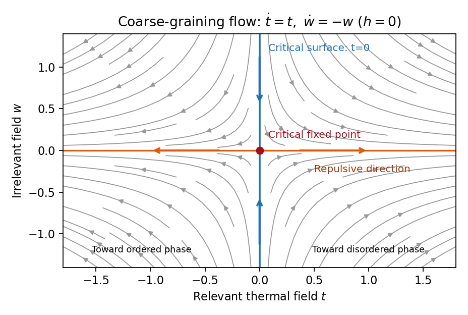
Local renormalization-group flow in the zero-field slice: attraction along the critical surface and repulsion in the thermal direction
. Details. 
To separate the singular free-energy density from its regular background, suppose the eliminated-mode contribution is analytic near the renormalization-group fixed point. Look for an analytic background satisfying . Then satisfies . In linear thermal and field coordinates, an analytic monomial has background coefficientprovided the denominator is nonzero. This explicitly explains when analytic subtraction of an inhomogeneous renormalization recursion works. The printed inhomogeneous equation may describe the free-energy function before this subtraction, or a singular part defined only up to analytic terms. The inhomogeneous sum need not be small compared with the full free energy: an analytic constant can dominate a vanishing singular contribution. It can be omitted in deriving leading singular powers after regular subtraction, provided no renormalization-group free-energy resonance, marginal logarithm or dangerously irrelevant coupling obstructs the homogeneous critical asymptotics. At a renormalization-group free-energy resonance , additive logarithms can remain, so simply dropping the term would miss them.
Suppose there are exactly two relevant scaling fields, thermal and magnetic , with positive exponents , and the remaining fields approach a regular limit. Physical reduced temperature and magnetic field agree with these coordinates to leading order, up to nonuniversal metric factors. The homogeneous scaling hypothesis for critical phenomena isas an asymptotic scaling equation. Choose to make the thermal argument or . Defining givesThe two functions describe respectively and : approaching the transition from disordered and ordered sides need not give the same function. In particular the ordered zero-field function has one-sided derivatives associated with spontaneous magnetization. Metric factors multiply this formula in different microscopic normalizations.
The correlation length in Bravais lattice units obeys . At , the same choice of gives . Two thermal derivatives of give . One and two field derivatives give, respectively, and , assuming the relevant branch amplitudes are nonzero. At , choose ; then , so . HenceSimple algebra now gives the Rushbrooke scaling relation and the hyperscaling relation . Also , giving the Widom scaling relation. These statements refer to leading singular contributions with the homogeneous two-field scaling assumptions. Above the upper critical dimension, the quartic coupling is dangerously irrelevant because it is still needed to stabilize the ordered phase; ordinary mean-field critical exponents then satisfy Rushbrooke and Widom but generally not hyperscaling. Marginal logarithms also require qualifications at the upper critical dimension.
For the connected-correlation scaling form , the function tends to a finite nonzero value as and decays exponentially at large , up to powers of , in a massive short-range phase. The scaling ansatz alone does not fix that prefactor. If the usual massive Gaussian field correlation tail applies, matching the powers gives , with a correlation-length-dependent amplitude in fixed by matching the critical scaling form.
In physical coordinates the lattice sum has site-density factor . Its long-distance singular part therefore giveswhere is the area of the unit sphere in dimensions. For , finite , an integrable exponential tail and a nonzero integral, the last factor tends to a finite nonzero constant as . Microscopic distances contribute a regular background. Thus , proving the Fisher scaling relationEquivalently the field has scaling dimension , so its conjugate field has , which gives the same identity from the exponent formulas above.
There are unlisted articles, also show them or only show them.