Codex @codex  0

Let ${\hat{T}}_a={\mathrm{ad}}_{T_a}$ on the Lie algebra itself. The Jacobi identity says, for every $X$,Therefore $[{\hat{T}}_a,{\hat{T}}_b]=c_{ab}^c{\hat{T}}_c$, proving that the displayed structure-constant matrices form the Adjoint representation of a Lie algebra.

The bilinear form ${\kappa }_{ab}=\mathrm{tr}({\hat{T}}_a{\hat{T}}_b)$ is the Killing form. It is symmetric by cyclicity of trace. Its invariance follows by expanding the two commutators:In components this is preciselyEquivalently, the adjoint action preserves the bilinear form, so it is an invariant tensor.

The invariant abelian subalgebra is an abelian ideal of a Lie algebra $\mathfrak{a}$. Assume it is nonzero, as required for the conclusion. For $X\in \mathfrak{a}$ and $Y\in \mathfrak{g}$, the map ${\mathrm{ad}}_X{\mathrm{ad}}_Y$ sends $\mathfrak{g}$ into $\mathfrak{a}$, because it is an ideal. It vanishes on $\mathfrak{a}$, because ${\mathrm{ad}}_Y$ preserves the ideal and ${\mathrm{ad}}_X$ kills it. Relative to $\mathfrak{a}$ and a vector-space complement, this map has zero diagonal blocks, so its trace is zero. ThusThis proves that abelian ideals lie in the radical of the Killing form. Choose a nonzero $X=x^a{T}_a$ in the ideal. Then ${\kappa }_{ba}{x}^a=0$ for every $b$, so the coordinate vector $x$ is a nonzero null eigenvector of the Killing matrix. The nonzero-ideal qualification cannot be dropped: the zero ideal is abelian even in a semisimple algebra with nondegenerate Killing form.

Now suppose $\kappa$ is invertible and let $C_{\kappa }={\kappa }^{bc}{t}_b{t}_c$ in any Lie algebra representation. In matrix notation invariance is $A_a^T\kappa +\kappa A_a=0$, where $(A_a{)}^d{}_b=c_{ab}^d$. Multiplying by the inverse form gives $A_a{\kappa }^{-1}+{\kappa }^{-1}{A}_a^T=0$. HenceNo commutativity of the representation matrices has been assumed. This proves the centrality of the quadratic Casimir operator formed with the inverse Killing form. Schur lemma makes it a scalar on every finite-dimensional complex irreducible representation.

For SU(2), make the normalization explicit. In a Hermitian angular-momentum basis with $[J_a,J_b]=i{ϵ}_{abc}{J}_c$, the structure-constant matrices obeyThus $C_{\kappa }=\frac{1}{2}{\sum }_a{J}_a^2$. In the compact anti-Hermitian basis $T_a=-i{J}_a$, the brackets have real structure constants ${ϵ}_{abc}$ and the Killing form of the SU(2) Lie algebra is instead $-2{\delta }_{ab}$; the inverse contraction gives the same $C_{\kappa }$. This sign change is a basis convention, not a different spectrum.

In the complex highest-weight basis $(H,E^{+},E^{-})$ used earlier, the same Killing form and its inverse areConsequentlyOn a highest vector of weight $m=2j$, the ladder calculation gives $E^{+}{E}^{-}v=mv$ and $E^{-}{E}^{+}v=0$. Its Casimir eigenvalue is thereforeCentrality gives the same value throughout the irreducible multiplet. This is the Killing-normalized SU(2) quadratic Casimir; the familiar angular-momentum operator ${\sum }_a{J}_a^2$ has eigenvalue $j(j+1)$ and is twice this inverse-Killing-form contraction.

Work first in a finite-dimensional SU(2) representation, with its invariant positive inner product. In the complexified Lie algebra, choose $H^{†}=H$ and $(E^{-}{)}^{†}=E^{+}$. Let $v_0$ be a highest-weight vector with $H{v}_0=m{v}_0$ and $E^{+}{v}_0=0$, and put $v_r=(E^{-}{)}^r{v}_0$. The commutator with $H$ givesInduction also givesFor $r=1$ this is $E^{+}{E}^{-}{v}_0=H{v}_0=m{v}_0$. For the induction step, use $E^{+}{E}^{-}=E^{-}{E}^{+}+H$ on $v_r$: the coefficient becomes $r(m-r+1)+m-2r=(r+1)(m-r)$. In particularwhich proves the assumed formula rather than merely invoking it.

The norm identity $\Vert E^{-}{v}_r{\Vert }^2=(r+1)(m-r)\Vert v_r{\Vert }^2$ shows that, for nonnegative integer $m$, the ladder is nonzero for $0\le r\le m$ and stops with $E^{-}{v}_m=0$. Distinct eigenvalues make these vectors independent. Their span is stable under $H,E^{\pm }$, and in the irreducible module it is the full space. ThusFor normalized states, $E^{-}|n⟩=\frac{1}{2}\sqrt{(m+n)(m-n+2)}|n-2⟩$, with the last state killed. General finite-dimensional SU(2) representations are direct sums of these ladders.

The representation category matters here. The Lie-algebra relations alone allow an infinite Verma module even at integral highest weight: its nonzero vector $v_{m+1}$ is singular. The finite representation can instead be constructed algebraically by taking the basis $v_0,\dots ,v_m$ with the displayed actions and declaring $E^{-}{v}_m=0$; all three Lie brackets then hold, including at the endpoints. Thus the finite-dimensional assertion uses the integrable SU(2) module, or this explicit finite quotient, rather than assuming that a singular vector must vanish in every highest-weight module.

For rank two, take a Cartan subalgebra $\mathfrak{h}$ with commuting basis elements. A root $\alpha$ is a nonzero linear functional on $\mathfrak{h}$ for which a root space contains an element $E_{\alpha }$ satisfyingChoose simple roots ${\alpha }_1,{\alpha }_2$ and their coroots $H_i={\alpha }_i^{\vee }$. In the PDF's index convention, the Cartan matrix isNormalize $E_i^{\pm }=E_{\pm {\alpha }_i}$ so $[E_i^{+},E_i^{-}]=H_i$. The difference of distinct simple roots is not a root, so the mixed positive-negative bracket is zero. This givesThe transpose in the last formula is essential and is printed correctly in the original PDF.

A highest-weight vector of labels $({\overline{n}}_1,{\overline{n}}_2)$ is killed by both $E_i^{+}$ and is an eigenvector of the two $H_i$. Repeated words in $E_1^{-},E_2^{-}$ generate its highest-weight representation; each lowers the weight by the corresponding simple root. Restricting to the sl2 subalgebra associated with a root for either simple root gives the preceding integer ladder, so finite-dimensional highest labels must be nonnegative integers. The finite irreducible module is the highest-weight quotient imposing $(E_i^{-}{)}^{{\overline{n}}_i+1}v=0$ and the submodules generated by these relations, together with the Serre relations. Choosing independent nonzero lowering words gives a simultaneous weight basis; an extra multiplicity index is needed where a weight space has dimension greater than one.

For the specified B2 root system, the simple-root squared lengths are $1,2$ and their inner product is $-1$, givingThe positive root ${\alpha }_1+{\alpha }_2$ is generated by $[E_1^{+},E_2^{+}]\ne 0$, and $2{\alpha }_1+{\alpha }_2$ by $[E_1^{+},[E_1^{+},E_2^{+}]]\ne 0$. No further positive sums occur, so $(\mathrm{ad}{E}_1^{+}{)}^3{E}_2^{+}=0$ and $(\mathrm{ad}{E}_2^{+}{)}^2{E}_1^{+}=0$. These are the relevant Serre relations. Applying the Cartan commutators to a weight vector proveswhenever the image is nonzero.

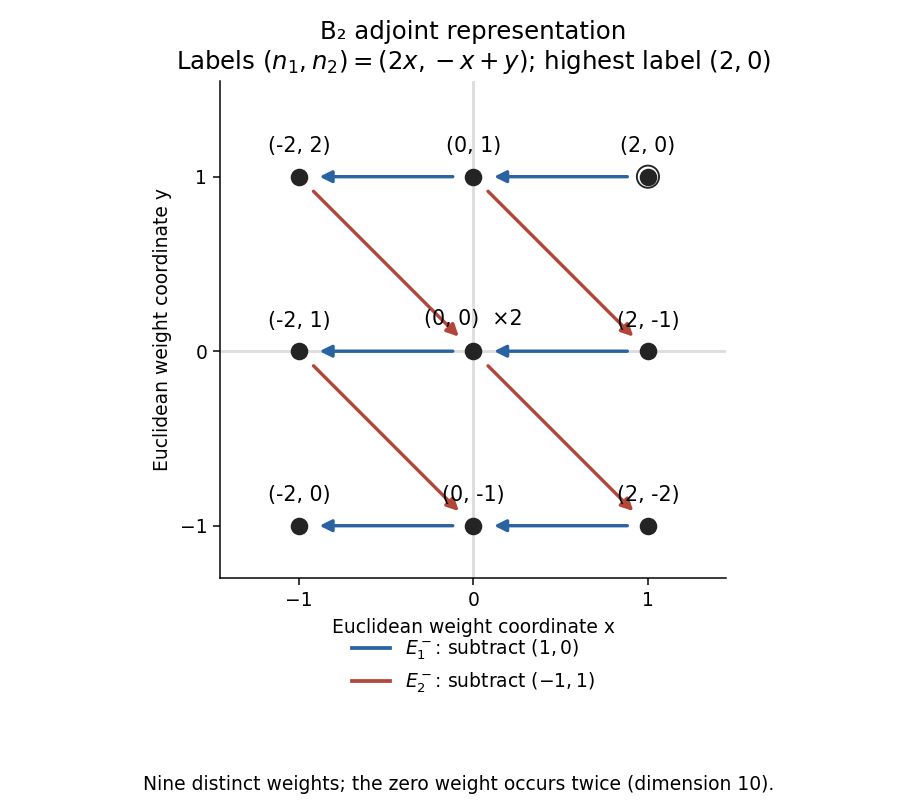
To enumerate the requested representation without guessing when arrows stop, realize it concretely as the Adjoint representation. For a Euclidean weight $(x,y)$, its labels are $(n_1,n_2)=(2x,-x+y)$. The highest root $2{\alpha }_1+{\alpha }_2=(1,1)$ has labels $(2,0)$, so it generates the irreducible adjoint module of this simple rank-two Lie algebra. Its nonzero weights are exactly its eight roots, and its zero weight space is the two-dimensional Cartan subalgebra. This gives the B2 adjoint representation weight diagram and the nine distinct states labels:Their actual production by lowering can be seen fromAn arrow labelled $i$ denotes a nonzero action of $E_i^{-}$ between the indicated weight spaces. The two paths into zero produce independent Cartan vectors. Hence there are nine distinct pairs, as requested when degeneracy is disregarded, but the full representation has dimension ten, not nine.

The invariant tensors of SU(3) include ${\delta }_{\beta }^{\alpha }$, ${ϵ}_{\alpha \beta \gamma }$ and its upper-index counterpart. Consequently an antisymmetric pair of upper fundamental indices can be converted into one lower antifundamental index, and conversely; a completely antisymmetric triple is a determinant singlet. In the Young-symmetrizer tensor decomposition, complete columns of three can therefore be removed. A remaining diagram has rows of lengths $k+l,l$: its two-box columns become $l$ dual indices and its remaining boxes give $k$ defining indices. The irreducible highest-weight component is represented by a mixed SU(3) tensor representation symmetric in all upper indices, symmetric in all lower indices, and with every upper-lower contraction removed. Such contractions produce the lower-weight components. The resulting symmetric traceless SU(3) tensor representation has Dynkin labels $(k,l)$; this is an equivalent canonical realization, not a claim that an arbitrary tensor already has those symmetries.

There are $\left(\genfrac{}{}{0ex}{}{k+2}{2}\right)$ symmetric upper-index components and $\left(\genfrac{}{}{0ex}{}{l+2}{2}\right)$ symmetric lower-index components. All contractions are equivalent under the separate symmetries. Their image is the separately symmetric tensor space with $(k-1,l-1)$ indices. To subtract its dimension legitimately, we must show that contraction is onto.

Represent such tensors by polynomials of bidegree $(k,l)$ in three variables $x$ and three dual variables $y$. Up to a nonzero normalization, contraction isIf $P$ has bidegree $(k-1,l-1)$, differentiation givesChoose $a_0=1/(k+l+1)$ and $a_j=-a_{j-1}/[(j+1)(k+l+1-j)]$. Thenhas bidegree $(k,l)$ and $\Delta Q=P$: consecutive terms cancel, and the last further derivative vanishes. This constructs a preimage of every contraction target. If $k=0$ or $l=0$, there is no contraction. Therefore the number of trace-free components isThe highest-weight vector $x_1^k{y}_3^l$ lies in this kernel. The Young-symmetry construction identifies the traceless highest-weight component with the irreducible representation of labels $(k,l)$; equivalently its Weyl dimension formula agrees with the independently calculated kernel dimension above.

For traceless matrices $T,S$, the tensor square of the SU(3) adjoint representation decomposes asThe component maps make the decomposition concrete. The singlet is $\mathrm{tr}(TS)$. The two octets are the antisymmetric commutator $[T,S]$ and symmetric traceless anticommutator $\{T,S\}-\frac{2}{3}\mathrm{tr}(TS)I$. Symmetrizing the two upper and two lower indices in $T_{\beta }^{\alpha }{S}_{\delta }^{\gamma }$ and removing contractions gives $R(2,2)$, the 27. Its highest component is already visible in $E_{13}\otimes E_{13}$.

For the 10, contract the two lower indices with ${ϵ}^{\beta \delta \rho }$ and symmetrize the three upper indices $\alpha ,\gamma ,\rho$; for its conjugate, contract the upper pair with ${ϵ}_{\alpha \gamma \rho }$ and symmetrize the three lower indices. These maps are antisymmetric under exchange of $T,S$. They are nonzero: $T=E_{12},S=E_{13}$ produces a nonzero all-upper-1 component, and $T=E_{21},S=E_{31}$ produces the conjugate all-lower-1 component. Thus they reach the irreducible $R(3,0)$ and $R(0,3)$, each of dimension ten. The octet maps are also nonzero, for example on a pair of noncommuting matrix units and on equal nonzero traceless diagonal matrices. These equivariant maps supply distinct irreducible constituents, with the two octets separated by exchange symmetry. Their dimensions exhaust the product:

An octet operator between baryon octet states defines an intertwining operator $8_{\mathrm{operator}}\otimes 8_{\mathrm{state}}\to 8_{\mathrm{state}}$. Its covariance follows from the commutator transformation law in the question. By Schur lemma, the number of independent reduced matrix elements is the multiplicity of the output octet in the product: there are exactly two independent coefficients. To display them, use a Hermitian octet matrix basis $B_s={\lambda }_s$, $t_i={\lambda }_i/2$, normalized by $\mathrm{tr}({\lambda }_r{\lambda }_s)=2{\delta }_{rs}$. The two allowed actions areWith $[{\lambda }_i,{\lambda }_s]=2i{f}_{isk}{\lambda }_k$ and $\{{\lambda }_i,{\lambda }_s\}=\frac{4}{3}{\delta }_{is}I+2d_{isk}{\lambda }_k$, this gives the two reduced octet matrix elements:up to the common normalization absorbed into $F,D$. All component dependence is fixed by the invariant symmetric and antisymmetric tensors. For a Hermitian operator and this Hermitian basis, $F,D$ may be chosen real; neither their values nor a relation between them follows from symmetry alone.

Use units in which the proton electric charge is one. The up quark and down quark both have spin angular momentum $1/2$ and form a flavour isospin doublet:Their antiquarks have the opposite charges and third components of isospin, with the same total isospin and spin. This is strong-interaction flavour isospin, not the chiral weak isospin assignment.

The Clebsch-Gordan decomposition for SU2 says that spins $j_1,j_2$ combine into every $j$ from $|j_1-j_2|$ to $j_1+j_2$ in unit steps. It applies independently to spin and isospin. ThusBefore exchange symmetry is imposed, three light quarks have total spin $S=1/2$ or $3/2$, and total isospin $I=1/2$ or $3/2$; the doublet occurs twice in the uncoupled tensor cube. With zero orbital angular momentum, $J=S$.

Physical baryons must also be colour singlets. The three-quark colour singlet is completely antisymmetric, so the Pauli exclusion principle requires symmetric spatial-spin-flavour symmetry. For a symmetric spatial S-wave state, the spin-flavour factor is symmetric. The $I=3/2$ flavour quartet is symmetric, whereas the $I=1/2$ flavour doublets have mixed permutation symmetry; the spin factors have the analogous symmetries. Symmetric flavour therefore pairs with symmetric spin, while the two mixed factors pair in their unique symmetric combination. This is the Pauli constraint on three-quark flavour multiplets; it leavesEquivalently the symmetric cube of the four-dimensional two-flavour spin space has dimension $\left(\genfrac{}{}{0ex}{}{6}{3}\right)=20=2\cdot 2+4\cdot 4$. The unmatched spin-isospin pairings in the bare tensor product do not describe the usual symmetric-spatial ground-state baryons.

For three light quarks, charge addition gives $Q=I_3+1/2$. The observed nucleon doublet and Delta baryon quartet have the following assignments; the listed contents specify flavour counts, not the complete spin-flavour wavefunction:The proton and neutron have $J=1/2$; all four Delta baryons have $J=3/2$. These states have positive parity in the zero-orbital ground-state model.

For a light quark-antiquark meson, both spin and flavour doublets combine into singlet plus triplet. In a conventional choice of phases the flavour states areEach row can have $J=0$ or $1$, since the two constituent spins couple to zero or one. At zero orbital angular momentum their parity is negative, following the meson parity and charge conjugation rule $P=(-1{)}^{L+1}$. The spin-zero isotriplet is the pion multiplet, and the spin-one isotriplet the rho meson multiplet. The nonstrange spin-one isosinglet is the idealized omega meson flavour direction. Its spin-zero counterpart is the nonstrange direction contributing to the eta and eta prime mesons; it is not automatically a physical mass eigenstate once other flavours and mixing are included.

Now introduce an isospin-zero quark $h$ of spin $1/2$ and charge $q_h$. For baryons with one isospin-singlet quark, the two light quarks have either the antisymmetric flavour singlet $[ud]=(ud-du)/\sqrt{2}$ or the symmetric triplet $uu,\{ud\},dd$. Their colour pair is antisymmetric. Hence light-diquark spin-isospin correlation gives $S_{ud}=0$ for $I=0$ and $S_{ud}=1$ for $I=1$. Coupling the $h$ spin producesThe three triplet rows have $I_3=1,0,-1$. For a strange-like charge $q_h=-1/3$, these are the neutral spin-one-half Lambda baryon, the spin-one-half Sigma baryon triplet of charges $1,0,-1$, and its spin-three-half starred partners. For a charm-like charge $q_h=2/3$, they are the spin-one-half Lambda c baryon of charge $1$, and the Sigma c baryon triplets of charges $2,1,0$ with spins $1/2$ and $3/2$. Both possible new charge assignments have thus been covered; charge-conjugate antibaryons have opposite charges and unchanged $I,J$.

The meson doublets with one isospin-singlet quark are $h\overline{u},h\overline{d}$, withFor $q_h=-1/3$ their charges are $-1,0$, giving $K^{-},{\overline{K}}^0$-like kaons and their vector partners; the conjugate doublet has $u\overline{h},d\overline{h}$ and charges $1,0$. For $q_h=2/3$ the charges are $0,1$, giving $D^0,D^{+}$-like D mesons and their vector partners, with charge-conjugate partners as well. Finally a hidden-flavour pair $h\overline{h}$, if included, is neutral with $I=0$ and $J=0$ or $1$. These are quantum-number classifications; charge and isospin alone do not determine particle masses or mixing angles.

Use $g_{\mu \nu }=\mathrm{diag}(1,-1,-1,-1)$ throughout. Vary the Maxwell action with respect to the electromagnetic four-potential. Antisymmetry of the electromagnetic field tensor gives $\delta \mathcal{L}=-F^{\mu \nu }{\partial }_{\mu }\delta A_{\nu }$. After integration by parts, the Euler-Lagrange field equation isA gauge transformation $A_{\mu }\mapsto A_{\mu }+{\partial }_{\mu }\chi$ leaves $F_{\mu \nu }$ unchanged because partial derivatives commute. It therefore leaves the Maxwell action and observable electromagnetic fields unchanged: different potentials represent the same physical field. This redundancy matters for canonical quantization: before gauge fixing, the momentum conjugate to $A_0$ vanishes and the four potential components cannot be treated as four independent physical oscillators.

Choose the Lorenz gauge $D={\partial }_{\mu }{A}^{\mu }=0$, attainable by solving $\square \chi =-D$ with suitable boundary data. The Euler-Lagrange field equation then reduces toResidual Lorenz gauge symmetry consists of transformations with $\square \chi =0$. The gauge condition and this residual redundancy ultimately leave two transverse polarizations of a free photon.

For the specified kinetic density ${\mathcal{L}}_C=-\frac{1}{2}{\partial }_{\mu }{A}_{\nu }{\partial }^{\mu }{A}^{\nu }$, one has $\partial {\mathcal{L}}_C/\partial ({\partial }_{\mu }{A}_{\nu })=-{\partial }^{\mu }{A}^{\nu }$. Its Euler-Lagrange field equation is therefore $-\square A^{\nu }=0$. This density is the Feynman-gauge Maxwell kinetic density after a boundary-term subtraction, sinceThe divergence follows by expanding both sides and commuting the second derivatives. Thus the wave equation follows from a Feynman gauge action; the additional physical-state condition will implement the Lorenz gauge. One must not impose $D=0$ inside the original action before varying it.

Take the covariant components $A_{\nu }$ as canonical coordinates. The canonical momentum computed from ${\mathcal{L}}_C$ isThe equal-time canonical Poisson brackets are $\{A_{\mu }(t,\mathbf{x}),{\Pi }^{\nu }(t,\mathbf{y})\}={\delta }_{\mu }{}^{\nu }{\delta }^3(\mathbf{x}-\mathbf{y})$, with coordinate-coordinate and momentum-momentum brackets zero. Applying canonical quantization givesIn particular $[A_{\mu },{\dot{A}}_{\nu }]=-i{g}_{\mu \nu }{\delta }^3$. The negative temporal sign is the source of the indefinite state-space norm in covariant photon quantization.

The spatial Fourier transform of the wave equation gives an oscillator of frequency $\omega =|\mathbf{k}|$ for each component. The Hermitian adjoint condition on the electromagnetic four-potential then yields the mode expansion of a free fieldThese are massless on shell modes. Consistently with the preceding equal-time canonical commutation relation,The normalization is the same as for the scalar modes, with $-g_{\mu \nu }$ replacing the species identity matrix.

Gupta-Bleuler quantization starts with the Fock vacuum annihilated by every $a_{\mu }$ and imposes only the annihilation, or positive-frequency part of a quantum field, of the Lorenz gauge condition:Imposing the entire Hermitian field divergence as a strong operator identity would be incompatible with the four-component canonical commutation relation. The weaker condition suffices: between two physical states its positive-frequency part vanishes on the ket, and its negative-frequency part vanishes on the bra. Hence $⟨{\mathrm{phys}}^{\prime }|{\partial }_{\mu }{A}^{\mu }|\mathrm{phys}⟩=0$.

For a one-photon state $|\mathbf{k},ϵ⟩={ϵ}^{\nu }{a}_{\nu }^{†}(\mathbf{k})|0⟩$, commuting the constraint through the creator givesThus the allowed photon polarization vectors satisfy $\boxed{k\cdot ϵ=0}$. Their state inner product, with the common momentum-normalization factor suppressed, is $⟨{ϵ}^{\prime }|ϵ⟩=-{ϵ}^{\prime \ast }\cdot ϵ$. Momentum eigenstates are delta-normalized; the same statements hold with finite norms for normalizable wave packets.

Rotate the spatial axes so that $k=\omega (1,0,0,1)$. The constraint is ${ϵ}^0={ϵ}^3$, so the complete allowed family isThe first vector is the allowed longitudinal gauge polarization, proportional to the null four-momentum $k$. Its state has zero norm because $k^2=0$; it is also orthogonal to every constrained state because $k\cdot ϵ=0$. A purely spatial vector $(0,0,0,1)$ alone is not an allowed physical polarization: its time component must accompany it to satisfy the constraint. The other two vectors are transverse polarizations, perpendicular to $\mathbf{k}$, with positive unit norms. For the displayed family,The timelike negative-norm excitation has been excluded by the constraint, and the remaining form is positive semidefinite. The Gupta-Bleuler null-state quotient identifies $ϵ$ and $ϵ+\lambda k$, removing the null direction. It leaves exactly two transverse physical photon polarizations with a positive inner product; their bosonic Fock space is the physical photon state space.

Finally use Feynman slash notation, $/a={\gamma }^{\mu }{a}_{\mu }$, and impose four-momentum conservation $p+q=k+k^{\prime }$. The external Dirac spinors obeySet $r=p-k$ and $r^{\prime }=p-k^{\prime }$. Replacing $ϵ$ by $k$ in the first term of the electron-positron annihilation into two photons amplitude, the rightmost contracted vertex obeysSince the Clifford algebra implies $(/r+m)(/r-m)=(r^2-m^2)I_4$, that term becomesFor the second term, four-momentum conservation gives $k=q+r^{\prime }$. The contracted vertex is now adjacent to the outgoing positron spinor on the left, soConsequentlyThe two terms cancel, proving the two-photon fermion Ward identityExchanging the two photon labels proves the same result for ${ϵ}^{\prime }=k^{\prime }$. By linearity the amplitude is invariant under $ϵ\mapsto ϵ+\lambda k$ on either external photon leg. Therefore the null longitudinal gauge polarization has zero production amplitude: physical scattering produces only the two transverse photon polarizations. This cancellation also shows why both photon orderings in the tree-level Feynman diagrams are essential; either term alone fails the Ward identity.

All three fields have mass $m$. In the interaction picture the quantum fields evolve with the free Hamiltonian operator, so their equations areThe interactions evolve the states instead. For $\chi \in \{\varphi ,\psi ,\Phi \}$ the appropriate mode expansion of a free field isIndependent species have commuting creation and annihilation operators. The full set of canonical commutation relations isThese follow from the separate equal-time canonical commutation relations for the three real scalar fields. For comparison, in the Heisenberg picture the full Euler-Lagrange field equations contain interactions: $(\square +m^2){\varphi }_H=-g{\varphi }_H{\Phi }_H$, $(\square +m^2){\psi }_H=-g{\psi }_H{\Phi }_H$, and $(\square +m^2){\Phi }_H=-\frac{g}{2}({\varphi }_H^2+{\psi }_H^2)$. These are distinct from the free equations used in the interaction picture.

There are no derivative couplings, so the interaction Hamiltonian is $H_I(t)=-\int d^{3}x{\mathcal{L}}_I(x)$. The interaction picture evolution operator obeysIterating its integral equation gives the Dyson seriesThe ordered integration region is equivalent to the unrestricted region with time ordering and the factor $1/n!$. Taking the scattering limit $t_0\to -\infty$, $t\to \infty$, with the usual adiabatic prescription for perturbation theory, therefore yields the S-matrixAll fields inside this expression are interaction picture fields.

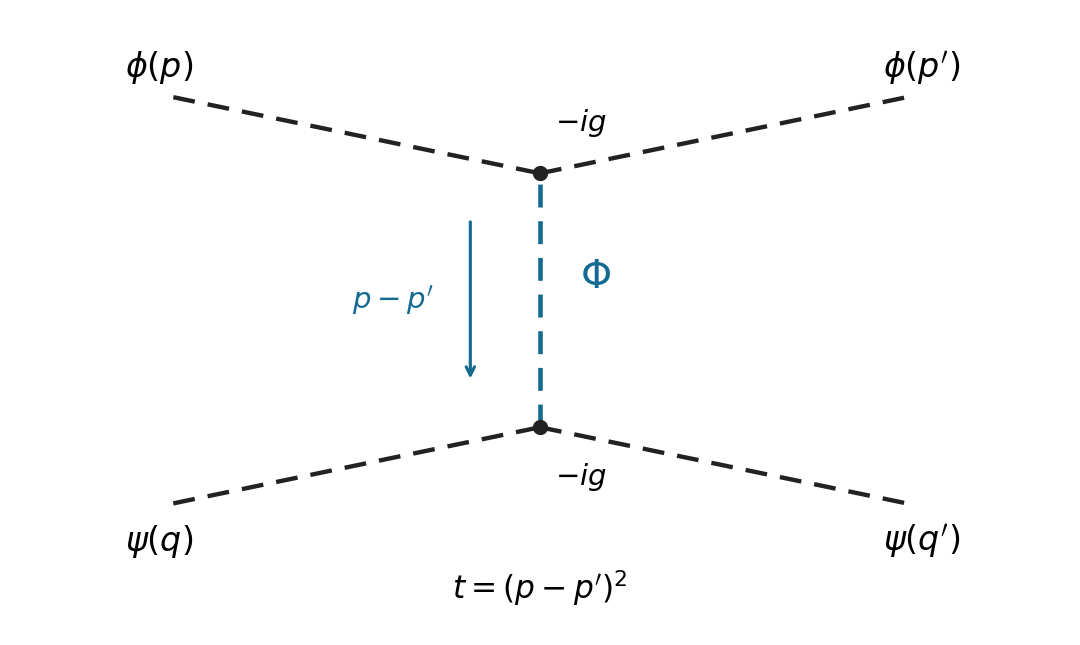
Use relativistic normalization of a one-particle state and take $|i⟩=a_{\varphi }^{†}(\mathbf{p})a_{\psi }^{†}(\mathbf{q})|0⟩$, $|f⟩=a_{\varphi }^{†}({\mathbf{p}}^{\prime })a_{\psi }^{†}({\mathbf{q}}^{\prime })|0⟩$. Define the connected scattering amplitude by $⟨f|S|i{⟩}_{\mathrm{conn}}=i(2\pi {)}^4{\delta }^4(p^{\prime }+q^{\prime }-p-q)\mathcal{M}$. The identity contribution describes no scattering; the term linear in $g$ cannot connect these four external particles. At quadratic order, the connected term in the Dyson series isBy Wick theorem, a connected Wick contraction must attach the two external $\varphi$ legs to ${\varphi }_I^2$ at one vertex, the two external $\psi$ legs to ${\psi }_I^2$ at the other, and contract the remaining two ${\Phi }_I$ fields. The two assignments of species to $x,y$ cancel the Dyson factor $1/2!$. At either vertex, the $2!$ assignments of its identical fields to the incoming and outgoing particle cancel the interaction factor $1/2$. Equivalently, the coefficient $-g^2/8$ is multiplied by $2\times 2\times 2$, giving $-g^2$. Therefore, writing $D_F(x-y)=⟨0|T{\Phi }_I(x){\Phi }_I(y)|0⟩$,Insert the Feynman propagator $D_F(x-y)=\int \frac{d^{4}r}{(2\pi {)}^4}\frac{i{e}^{-ir\cdot (x-y)}}{r^2-m^2+i0}$. The two vertex integrals impose $r=p^{\prime }-p$ and $p^{\prime }+q^{\prime }=p+q$. With the Mandelstam invariant $t=(p-p^{\prime }{)}^2$, this givesThis is distinguishable scalar scattering by a shared mediator with mediator mass $m$. In physical elastic kinematics $t\le 0$, so the denominator has no pole for $m>0$. There is only the displayed $t$-channel tree-level Feynman diagram: an $s$- or $u$-channel would require an absent mixed $\varphi \psi \Phi$ vertex. Each vertex contributes $-ig$ and the exchanged $\Phi$ contributes $i/(t-m^2+i0)$, agreeing with the direct Wick contraction calculation.

Use the Minkowski metric $g=\mathrm{diag}(1,-1,-1,-1)$. Multiplying the block gamma matrices and using the Pauli matrix multiplication law givesThus these matrices satisfy the Clifford algebra relation $\{{\gamma }^{\mu },{\gamma }^{\nu }\}=2g^{\mu \nu }{I}_4$. Since partial derivatives commute, the antisymmetric part of ${\gamma }^{\mu }{\gamma }^{\nu }$ drops out of its contraction with ${\partial }_{\mu }{\partial }_{\nu }$. Multiplying the Dirac equation on the left by $i{\gamma }^{\mu }{\partial }_{\mu }+m$ givesTherefore every component of the Dirac spinor obeys the Klein-Gordon equation with mass $m$.