
Past exam of the mathematics course of the University of Cambridge 2003 iii Paper 49 4 Solution Created 2026-10-03 Updated 2026-10-14
A renormalized coupling is defined by a subtraction or reference condition at a renormalization scale . Radiative corrections contain logarithms of momentum scales relative to , so changing the reference scale changes the named coupling while leaving physical observables unchanged. Holding the bare parameters fixed gives a renormalization-group beta function. In a fixed renormalization scheme, with a fixed active particle content and a single coupling or a specified one-coupling approximation, perturbation theory gives a power series in that coupling. Its coefficients depend on the fields, representations and scheme; beyond the universal leading coefficients they need not be scheme independent. A theory with several couplings generally has coupled beta functions, so the question's scalar equation is schematic rather than literally the form of every quantum field theory. Also , which fixes factors of two.
For the stated leading equation let . Differentiating the reciprocal gives , henceFor , defineThen , givingThis is one-loop running of the strong coupling, with here normalized exactly as in the source equation. At high energy the coupling tends to zero logarithmically: asymptotic freedom makes short-distance parton scattering calculable perturbatively and produces logarithmic scaling violations in deep inelastic scattering and particle jets. As the scale approaches from above, the coupling becomes large and the perturbative approximation fails. Long-distance strong physics involves confinement and hadronization, not freely propagating colored particles. The apparent one-loop pole is not a proof of confinement, and the negative formal continuation below is not a physical coupling. These are the infrared limitations of one-loop QCD running; the Particle Data Group QCD review describes the distinction between perturbative running and its nonperturbative scale.
The expected rough QCD scale is of order a few hundred MeV, comparable to the inverse hadronic length scale . This is an empirical dimensional estimate, not a numerical deduction from alone. Indeed the integration constant also requires a measured reference coupling. Its precise value depends on flavor number, perturbative order and renormalization scheme.
For , the same integrated solution instead increases with energy and has its perturbative Landau pole atThe coupling decreases toward the infrared in this approximation; toward the ultraviolet, perturbation theory ceases to be reliable before reaching the pole. For the self-coupling-dominated Higgs approximation, use the conventional Higgs potential . ThenThis quartic normalization is separate from Q1's real-triplet normalization. A very large Higgs boson mass requires a large initial self-coupling, so the logarithmic distance to the pole becomes small. Requiring a weakly coupled Standard Model up to a high scale demands approximatelywith a stronger practical margin to keep the evolved coupling perturbative. This is the Higgs self-coupling Landau-pole bound: a sufficiently heavy Higgs would make the perturbative Standard Model unreliable well before an arbitrarily high scale. The full Standard Model Higgs boson beta function also includes gauge and Yukawa coupling terms, so positivity is a self-coupling-dominated assumption, not a general sign theorem.
For the requested bottom threshold, take the physical color number . In the source normalization,Continuity of the leading coupling at givesDivide by to find . Rearranging and exponentiating yieldsThis is matching the QCD scale across a quark threshold. The named integration constant changes when the beta coefficient changes; the matched coupling itself stays continuous at leading order. If the number of colors were kept arbitrary, the exponent would instead be ; the printed exponent therefore uses .
Past exam of the mathematics course of the University of Cambridge 2003 iii Paper 49 3 Solution Created 2026-10-03 Updated 2026-10-14
Let , so . Direct multiplication of the Pauli matrices gives , equivalently . For this impliesTherefore transforms as the same weak fundamental representation doublet as , while complex conjugation reverses its hypercharge to . This is the Higgs conjugate doublet. The Yukawa coupling product is an singlet, and its hypercharges add toIt is consequently gauge-invariant and can supply an up-quark mass.
In unitary gauge, . Writing for the full arbitrary coefficient of the Yukawa coupling term, its physical form isA one-generation field rephasing makes the mass positive, and its Higgs boson coupling is . The printed Yukawa expression has an additional trailing after which is never defined. If it denotes a constant, absorb it into ; in the conventional dimensionless Yukawa notation without that factor, . It does not affect the gauge-transformation argument.
For three families, use a singular value decomposition of the two mass matrices: and , with positive diagonal entries. The original left-handed weak current then becomes a current between mass eigenstates withA complex matrix has eighteen real parameters, and imposes nine independent real conditions, leaving nine. A generic unitary matrix can be built from three complex plane rotations and three diagonal phases: each plane rotation supplies one angle and one phase. Thus these are three rotation angles and six phases. Rephase each of the six Dirac quark mass eigenfields, applying the same phase to its two chiralities so the diagonal masses stay real. A common phase changes no entry of , leaving five effective rephasings. Removing five of the six phases leaves three angles and one physical phase. This CKM parameter counting assumes generic nondegenerate masses; degeneracies give additional basis freedom.
Exactly massless neutrinos have an arbitrary unitary flavor rotation that changes no mass term. After diagonalizing the charged-lepton mass matrix, choose the neutrino basis with the same left-handed rotation. The apparent lepton charged-current mixing matrix becomes the identity. Thus mixing of exactly massless neutrinos is removable; it is not an analogue of physical CKM mixing.
For the requested CP symmetry calculation, write . The supplied charge conjugation transformations, with the fermion-reordering sign, giveFor , use and the given gamma matrix relation to obtainUnder parity, the current acquires the Lorentz parity matrix and becomes . Under charge conjugation the charged vector also changes sign and becomes its conjugate. The two minus signs cancel, and the parity matrices cancel in the contracted operator. ConsequentlyWith , the interaction is . Thereforewith the transformed density evaluated at . This is the CP transformation of a charged quark current.
Physical noninvariance requires a phase that cannot be removed by quark rephasings. The invariant quartetis the Jarlskog invariant, where and in the standard three-angle parametrization. If , no allowed row/column phases can make the matrix real, and the charged-current interaction violates CP symmetry. For example all three angles with give .
The printed noninvariance claim is conditional on a nonzero physical phase. Arbitrary Yukawa matrices do not force it: , or any real CKM matrix, gives a CP-invariant charged-current interaction. The correct statement is generic CP violation when the irreducible phase is nontrivial, as explained by quark rephasing and CP conservation.
Finally a right-handed neutrino has gauge representation . Its Lorentz-invariant same-chirality bilinear with the field obtained by charge conjugation is therefore a gauge singlet and permits a Majorana mass term, conventionallyThe factor is the usual convention for a field paired with itself; it may be absorbed into the printed coefficient. A Higgs Yukawa interaction can independently give a Dirac mass term. The Majorana term violates lepton number by two units but preserves the gauge symmetries. Corresponding terms for the other charged Standard Model fermions carry nonzero electric charge, and quarks also carry nontrivial color charge. Thus this gauge-invariant right-handed neutrino Majorana mass is allowed while those charged-fermion analogues are forbidden. Merely introducing a right-handed neutrino permits mass; vanishing mass coefficients would still leave it massless.
Past exam of the mathematics course of the University of Cambridge 2003 iii Paper 49 2 Solution Created 2026-10-03 Updated 2026-10-14
Use the source convention , with electric charge measured in units of the positron charge. Expanding the covariant derivative in the fermion kinetic term gives interaction . Substituting the given neutral-field rotation, the coefficient of isThe photon coefficient is , with . For a Dirac field, acts only on its left-handed component. ThusThe weak neutral current interaction consequently has the requested form, withThe electroweak representation and hypercharge table gives the following values for one generation:
These neutral-current vector and axial couplings use the source's vertex prefactor . They are twice the coefficients used with prefactor ; the latter convention must not be mixed into this calculation. For the neutrino, the chiral projector removes the inactive right-handed component automatically.
Set and suppress the species label. For outgoing momenta , the amplitude is, up to an irrelevant phase,The final-state spin sum is the Dirac trace of . Anticommutation of with the gamma matrices makes its symmetric partThe vector-axial cross term is proportional to the antisymmetric Levi-Civita symbol, so it contracts to zero with the symmetric massive vector polarization sum . Since , the symmetric tensor is transverse to as well. Only remains, andMultiplying by proves the massless fermion Z decay spin sum:
For the decay width, average over the three initial polarizations. Rotational invariance makes the integrated width the same for each initial spin state, so the massive-vector spin average is legitimate even for a single prepared polarization. In the rest frame, the delta functions in two-body Lorentz-invariant phase space leaveThis follows by setting and integrating ; the radial integration supplies a factor . HenceFor a quark species multiply by three colors, with strong-interaction radiative corrections when comparing with data. For one effectively massless active neutrino, , so .
The total resonance width contains visible charged-lepton and hadron decays plus . Thus the measured invisible contribution determinesEarly resonance measurements supported three light active neutrino species, with experimental uncertainties; the OPAL analysis of its 1989 data explicitly compares the three- and four-species predictions. Under the question's assumption that every possible family has a massless neutrino with ordinary weak couplings, this constrains the number of such families. The inference does not exclude additional neutrinos heavier than or gauge singlet sterile states with no ordinary coupling. This is light-neutrino counting from the Z width.
Past exam of the mathematics course of the University of Cambridge 2003 iii Paper 49 1 Solution Created 2026-10-03 Updated 2026-10-14
Assume and . The minima of the scalar potential have . Choose the vacuum expectation value . Its stabilizer subgroup consists exactly of matrices with , soThe continuous spontaneous symmetry breaking is and has two broken generators. For the full orthogonal group, the cross-product notation requires the gauge connection to transform in the adjoint, as an axial vector: . The scalar field transforms as the ordinary vector . This axial transformation of orthogonal gauge connections makes the stated covariant derivative transform correctly even for ; assigning an ordinary-vector transformation to the connection would fail.
Near this nonzero vacuum, unitary gauge removes the two angular Goldstone bosons and gives . PutThese are the physical charged gauge bosons, neutral massless gauge boson, and radial scalar field. Directly substituting into the original gauge field strengths givesThe scalar field kinetic term has no radial-vector cross term, because and lie in perpendicular internal directions. The complete physical gauge-scalar Lagrangian becomesFor each real vector the mass term is , while for the complex pair it is . Hence the adjoint triplet Higgs spectrum isThe radial scalar also has in the question's potential normalization. The two lost scalar modes supply the longitudinal polarizations of the massive vectors through the Higgs mechanism.
For the lepton kinetic terms let , , and denote the left neutral triplet entry by . The missing singlet is the perpendicular combinationIts overall sign is immaterial. The real orthogonal matrix is orthogonal, so the sum of the kinetic terms of and is with no mixed terms. Combining with the right triplet gives ordinary Dirac field kinetic terms for , and only a left-handed kinetic term for the massless neutrino. This is orthogonal completion of mixed neutral lepton kinetic terms. The heavy charged field is , as printed in the PDF, not the TeX's .
To compute the charge commutator, the canonical anticommutation relations implyThe quartic terms cancel on reordering the fermions. Thus well-defined normal-ordered integrated bilinears obey fermionic bilinear charge algebra, . Left/right mixed commutators vanish since .
In either triplet, writeThe displayed current has a factor two relative to the projected bilinears, since . Consequently its charges are and . The neutral combinations have canonical anticommutators because . Applying the matrix commutator giveswhere is the electromagnetic charge in the lepton sector. The neutrino, heavy neutral lepton and singlet contribute zero. This establishes triplet charged-current closure on electromagnetic charge, with the requested proportionality independent of normalization choices for the weak Noether charges. The PDF correctly writes ; the TeX repeats incorrectly. Equal-time algebra does not require conservation of the separate fermionic weak currents after symmetry breaking. For full gauge-theory charges, the corresponding charged-boson contributions must also be included.
Past exam of the mathematics course of the University of Cambridge 2003 iii Paper 48 3 i Created 2026-10-03 Updated 2026-10-14
Past exam of the mathematics course of the University of Cambridge 2003 iii Paper 48 1 Solution Created 2026-10-03 Updated 2026-10-14
Write the Hamiltonian operator as , with , and define the quantum-mechanical propagator by . Use intervals of length , endpoint coordinates , and the Trotter product formula. Inserting the completeness relations of the position eigenstates between the short-time factors givesNormalize momentum eigenstates by . The Gaussian integral over the intermediate momentum isThe square-root branch is fixed by continuation from . Consequently the precise time-sliced configuration-space path integral isThis formula defines the notation ; it is not an unnormalized infinite product of ordinary integrals. For real time take the boundary value from , , or the corresponding oscillatory-distribution limit. For a self-adjoint, bounded-below Hamiltonian operator under the usual product-formula hypotheses, the operator limit supplies the definition even where the coordinate kernel is a distribution. The discrete exponent approaches the action with kinetic term , and the prefactor is part of the functional measure. A different consistent slicing gives the same kernel for this separated kinetic-plus-potential Hamiltonian.
For the quantum harmonic oscillator, expand the action about a classical path , writing with homogeneous Dirichlet boundary conditions on . The only mixed term isThe boundary term vanishes and the Euler-Lagrange equation sets the remaining integrand to zero. Thus exactly, rather than only to quadratic approximation. Translation of each integrated coordinate has unit Jacobian determinant; in the continuum measure convention of the question this is . The classical-path factorization of a quadratic path integral follows:The fluctuation action, measure and boundary values depend on but not on . For real with the boundary-value classical path exists uniquely. At the conjugate times , generic endpoints admit no such path and the kernel is a delta distribution; the formula is interpreted by the same regulated boundary limit, not as an ordinary finite prefactor times a nonexistent classical solution.
Past exam of the mathematics course of the University of Cambridge 2003 iii Paper 47 4 Solution Created 2026-10-03 Updated 2026-10-14
Write both the input and output integer labels in most-significant-bit-first order, and . Factoring the Fourier phase over the bits of gives the product decomposition of a Fourier phase state:Here denotes the binary fraction ; the integer part of does not affect the phase.
Build a dyadic quantum Fourier transform circuit as follows. Process wires in that order. First apply a Hadamard gate to wire . Then, for each , apply the controlled phase gate with control wire and target wire . On a computational-basis state, every unprocessed control is still the bit , so wire becomesOnce a wire has been processed it is not touched by later stages. Reversing the order of the output wires gives exactly the Fourier product above. Agreement on every computational-basis state proves agreement as linear operators on all superpositions, even though the intermediate operation on a general input can create entanglement.
There are Hadamard gates and controlled phase gates. Output reversal may be treated as wire relabelling. If it must instead be implemented physically while using only the requested gate family, use swap operators. Each swap is three controlled-NOT gates, andThus the swaps use only Hadamard gates and Controlled-Z gates, which are controlled gates. An exact physical network haselementary gates from the stated family. This implements the positive-exponent Fourier transform with the correct output order in quadratic size. Omitting the output reversal without relabelling the wires would produce the reversed-order transform instead.
For the perturbation bound, the operator norm in the source is equivalently . It satisfies the triangle inequality, is unchanged by left or right multiplication by a unitary operator, and a unitary operator has norm one. The exact telescoping identity isIt follows by replacing one factor at a time; alternatively all intermediate products cancel in the sum. Taking the operator norm and using unitary invariance gives the quantum circuit gate-error telescoping boundThe original PDF assumes strict , so its strict conclusion is justified. If the hypothesis were weakened to a non-strict inequality, the conclusion would likewise be . The TeX aid misreads this hypothesis; the PDF resolves it.
Apply the non-strict version to each approximate unitary gate in the Fourier network. Extending a gate by the identity on other wires leaves its operator norm error unchanged. Including the physical swap decompositions, all gates are of the required type and can obey the stated accuracy. HenceWith exact output relabelling rather than physical swaps the numerator is just . The proof retains gate phases and makes no assumption of cancellation between coherent errors.
For every normalized input the output-state norm error is at most this same bound. If is any positive operator satisfying , the change in its measurement in quantum mechanics outcome probability is at most , where : expand the difference of the two expectations into two terms, each bounded by using the Cauchy-Schwarz inequality. Thus inverse-polynomial gate accuracy gives an inverse-polynomial total error, rather than requiring exponential precision in the number of qubits. For the phase gates this corresponds to specifying angles with bits of precision, since . This is a robustness statement for unitary gate approximations; it does not by itself correct quantum decoherence, correlated stochastic faults, or limitations of hardware connectivity.
Past exam of the mathematics course of the University of Cambridge 2003 iii Paper 47 3 Solution Created 2026-10-03 Updated 2026-10-14
Use the Hilbert-Schmidt inner product normalized by the dimension: . The identity and the three Pauli matrices are Hermitian, each has square , and each nonidentity Pauli matrix has zero trace. For distinct nonidentity indices, the Pauli matrix multiplication law gives , which is traceless. ThereforeThere are four such orthonormal operators, and the complex vector space of two-by-two matrices has dimension four. Hence they form an orthonormal basis. Taking the inner product of any with each basis element proves, for arbitrary complex and not just Hermitian ones,For example, if , its four coefficients are , , , and , respectively.
For the joint error, regard the two prescribed basis outputs as the columns of an environment-valued linear map. Its coefficient array in the usual output-row, input-column convention isThe source's other array is arranged as a column of the images of basis kets; it must not be mistaken for this coefficient array acting on an amplitude column. Applying the just-proved Pauli matrix expansion componentwise in any environment orthonormal basis gives the Pauli decomposition of a qubit-environment isometry:To check the potentially delicate sign of the Pauli Y gate coefficient, use and . The four terms then giveLinearity proves the expansion for every input pure state. The environment coefficient vectors need not be normalized or mutually orthogonal. Consequently this expansion includes coherent combinations of Pauli errors, rather than asserting that every quantum channel is a probabilistic Pauli channel.
For the recovery probability, use the usual independent-use interpretation of the given phase-flip channel: each of the three transmitted qubits has a Pauli Z gate error independently with probability . The phase-flip repetition code uses logical codewords and . The decoding Hadamard gates convert physical phase flips to bit flips because . We can then analyze the two decoding controlled-NOT gates and the final Toffoli gate directly, rather than assuming a recovery rule.
Let be the error bits after this basis conversion. For a logical basis input , the three data bits before inverse encoding are . The two controlled-NOT gates produceThe Toffoli gate flips the first wire when both of the last two bits are one. Its residual error isThe last two wires carry an error syndrome independent of . Thus this transformation preserves the amplitudes of an arbitrary superposition: zero or one phase error returns the original unknown qubit, while two or three phase errors leave the logical Pauli X gate applied to it. The probability of universally successful recovery is thereforeEquivalently, the decoded quantum channel is , with logical failure of the three-qubit phase-flip repetition code . For , the failure probability is below , since . A special input that is a Pauli X eigenstate is unchanged even by the residual logical error; this does not make the code correct that error on an unknown input. Its squared quantum fidelity with a particular pure input is . If the errors on different channel uses are correlated, the marginal probability alone is insufficient: the general universal success probability is the probability of at most one error.
Past exam of the mathematics course of the University of Cambridge 2003 iii Paper 47 2 Solution Created 2026-10-03 Updated 2026-10-14
The Walsh-Hadamard transform is the tensor product of one Hadamard gate on each qubit. Indeed,The network therefore consists of parallel Hadamard gates, with no interaction between wires. Applied to an all-zero quantum register, it produces the uniform quantum superposition of all input strings. This lets a Boolean quantum oracle act coherently on all those inputs; a subsequent operation can turn their relative phases into useful interference. It does not permit reading all oracle values from a single measurement in quantum mechanics.
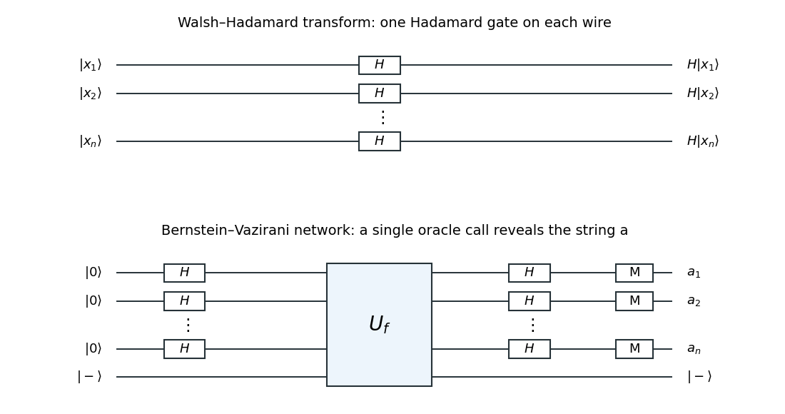
Parallel Hadamard gates and the one-query Bernstein-Vazirani network
. Details. 
For the supplied linear-phase input, the amplitude on output isEach factor is obtained by summing over the independent bit . This directly proves the relevant orthogonality of the binary Fourier phases, and yields the output state exactly.
For exact classical identification, query the Boolean function at the standard unit vectors: . Hence oracle calls suffice. They are also necessary in the worst case, even with adaptive queries: every answer supplies one binary linear equation in the unknown string. With fewer than queries, their coefficient matrix has matrix rank at most the number of queries, so its null space contains a nonzero string . The strings and give identical answers along that adaptive transcript and cannot both be identified correctly. Equivalently, a depth- binary decision tree has at most leaves and must distinguish possibilities. Thus the exact classical query count is . This concerns exact recovery, rather than allowing an arbitrary error probability.
The quantum network in the lower panel starts its data quantum register in and its answer ancilla qubit in , which can be prepared as . Apply Hadamard gates to the data wires, make one Boolean quantum oracle call, then apply Hadamard gates again to all data wires. Quantum phase kickback producesA computational-basis measurement of the data wires gives all bits of with certainty. This is Bernstein-Vazirani phase kickback: one quantum query, data Hadamard gates, and one answer-state preparation suffice. The answer ancilla qubit stays separate from the data at the output.
Past exam of the mathematics course of the University of Cambridge 2003 iii Paper 47 1 Solution Created 2026-10-03 Updated 2026-10-14
Take the Hadamard gate to be and the phase gate to be . This fixes the sign convention for the interference phase.
For the coherent quantum circuit, the successive quantum states areThe Born rule therefore gives the concise answer
With the stated quantum decoherence after the phase gate, the joint pure state before the last Hadamard gate isAfter that Hadamard gate, its environment coefficient at output zero is . Squaring its norm sums over every unobserved environment outcome, soThe Cauchy-Schwarz inequality gives . In this single-qubit interference with conditional environment states, is the interference visibility: orthogonal environment states erase the fringe, while a unit-modulus overlap shifts its phase without reducing visibility. The plus sign in follows from the specified overlap , rather than its complex conjugate.
If the same quantum decoherence occurs before the phase gate, the joint pure state is first . The phase gate then produces exactly the same state used above. Equivalently, the controlled environment interaction commutes with the diagonal phase gate. The probability is unchanged.
For the Deutsch algorithm, use the reversible Boolean quantum oracleThe algebraic oracle map printed in the source has its arguments misplaced: taken literally, it sends two distinct answer inputs to the same output for constant , so it cannot be a unitary operator. The corrected map above agrees with the diagram's input-control, answer-target arrangement. Put the answer qubit in . Since the Pauli X gate satisfies , quantum phase kickback givesWrite . Up to the irrelevant global phase , the input qubit acquires relative phase , so its ideal final computational-basis measurement returns : zero for a constant function and one for a balanced function.
Let the specified quantum decoherence occur in the interference portion between the two Hadamard gates. It commutes with the oracle's effective diagonal phase on the input, so the same analysis applies whether it occurs just before or just after the query. The two likelihoods areThus the diagram's usual zero-for-constant decision rule hasThis is the reliability for either promised class separately, with no prior needed. For equally likely classes, if is known to be negative, reversing the interpretation gives . A known environment phase can instead be compensated by the phase gate before the final Hadamard gate, giving success probability . In particular, gives no information and permits certainty after phase compensation. These refinements distinguish a shifted fringe from lost quantum coherence; with the unmodified diagram a phase shift alone can reverse the apparent answer. Quantum decoherence after the final Hadamard gate leaves its computational populations unchanged, so that different placement would not spoil the measured answer.
Past exam of the mathematics course of the University of Cambridge 2003 iii Paper 46 3 Solution Created 2026-10-03 Updated 2026-10-14
Changing the ultraviolet cutoff changes which fluctuations remain explicit. Integrating out a shell of Fourier modes shifts the coefficients of all symmetry-allowed operators and a field-independent constant. Hence the cutoff-dependent coefficients are chosen so that the remaining partition function and long-distance observables reproduce the same microscopic system. This is the Wilsonian coarse-grained statistical Hamiltonian; retaining only the printed operators is a local derivative expansion, not an exact closure.
In a massive symmetric phase, the quadratic long-wavelength inverse two-point function has the form . Its Landau scalar correlation length satisfies in this approximation. For canonical normalization of a scalar gradient term, set ; then the mass and quartic coefficients become and . With this normalization the infrared mass is the inverse correlation length, , within the massive quadratic or one-loop approximation. More generally the decay rate is a pole mass, whereas the zero-momentum inverse magnetic susceptibility is a curvature mass; an anomalous dimension or nontrivial momentum dependence can distinguish them. In the ordered phase one must first expand about a selected stable equilibrium magnetization, rather than identify a negative quadratic coefficient at the unstable origin with a squared inverse correlation length. Thus the intended mass identification includes a field normalization and a stable-phase qualification.
For momentum-shell renormalization group, split , retaining and eliminating . DefineTaking a logarithm gives the cumulant expansion of a coarse-grained free energy. For a centered fast Gaussian measure with , the first quartic cumulant isThe Wick contractions give a mass shift and an identity-operator contribution, while leaving the quartic term at this order. The second cumulant produces higher interactions and a quartic correction. After the length and field rescalings and , the gradient coefficient remains one, andThe one-loop shell mass renormalization in scalar quartic theory explicitly shows why the critical bare mass is shifted by fluctuations.
Assume short-range interactions, an analytic even local potential, a positive gradient coefficient, and a weak-coupling trajectory in the basin of the Gaussian fixed point. Above four dimensions the quartic interaction has negative engineering dimension and its dimensionless strength decreases under coarse graining; higher local powers and higher derivative terms also decrease. After absorbing analytic short-distance shifts into the coefficients, long-wavelength fluctuations are small compared with the ordered order parameter. The remaining coarse Landau free energy can therefore be evaluated at its stable saddle:The quartic stabilizer must still be retained for the ordered minimum even though it is dangerously irrelevant. Stationarity, , gives the ordinary Landau-Ginzburg theory and its mean-field critical exponents. This derives the saddle approximation from decreasing fluctuation strength under the stated RG assumptions; it does not assume that every exact coarse-grained functional becomes a quartic polynomial. Below four dimensions the quartic coupling grows, long-wavelength loop corrections cease to be small, and the argument fails. At four dimensions the interaction is marginal and generates logarithmic corrections. The tuned sextic theory has the analogous boundary at three dimensions.
Use a consistent Fourier transform pair for the connected correlation function:The printed forward-transform expression integrates over while leaving free; that integration variable is an error. The above convention resolves it and produces the loop measure used below. At zero magnetization, ; otherwise the disconnected product of expectations must be subtracted.
In the inverse-propagator identity used here, the truncated two-point function means the full one-particle-irreducible two-point vertex, including its free quadratic part. This convention differs from using “truncated” for a connected cumulant. To derive the inverse relation, introduce , and the effective action . Then and the chain rule gives . Since is the connected correlation function, translation invariance gives .
Now use canonically normalized coefficients, denoting the cutoff mass by and the renormalized infrared mass by . Choose the free propagator and put in the interaction as a quadratic counterterm. With the Euclidean self-energy convention in which an insertion changes the connected propagator by , the perturbative series beginsThe self-energy sums one-particle-irreducible loop insertions; the explicit mass counterterm is kept separate. Repeated insertions generate the geometric Dyson resummation, which explains why reducible chains occur in but not as independent terms in its inverse. Beyond one loop a momentum-dependent self-energy and wave-function renormalization must also be included.
At one loop the only quartic two-point graph is the tadpole diagram. At a vertex, attaching the two labeled external fields uses choices and contracts the remaining two fields together. The factor is . Equivalently this is the same quadratic term in the shell cumulant expansion above. ThusIt is positive for and independent of external momentum, so there is no one-loop gradient renormalization. The condition implies , henceThe cutoff is necessary: the unregulated integral is ultraviolet divergent for . Using the renormalized mass internally is a self-consistent one-loop organization, not an exact resummation of all critical fluctuations. With nonunit , this formula instead applies to , after canonical normalization of a scalar gradient term.
To test a linear thermal mass, approach the ordinary transition from the symmetric side and set . For the massless tadpole is infrared finite. Subtract its critical value, absorb regular temperature dependence of the coupling into a nonzero thermal coefficient , and write . The one-loop critical-mass subtraction giveswhereFor , is finite, so the bracket tends to a finite constant and is self-consistent. At ,and the growing logarithm obstructs an asymptotically constant linear coefficient at nonzero coupling. For , put to obtainThe divergent bracket then invalidates the assumed linear thermal mass. The radial critical-mass subtraction in dimensions three to five gives explicit checks of all three behaviors. For , the massless tadpole subtraction itself is infrared divergent; that failure of the Gaussian expansion does not prove absence of an interacting transition. Therefore the ordinary upper critical dimension is , with the unmodified Landau-Ginzburg theory asymptotically justified by this test only for . Exponents inferred by solving the self-consistent one-loop equation below four dimensions would not be exact interacting exponents.
For a tricritical point the renormalized quartic coefficient must be tuned to zero, and a positive sextic interaction stabilizes the order parameter. The gradient term gives the scalar field engineering dimension . A coefficient of therefore has dimension , which becomes marginal at . This gives . A direct Ginzburg criterion reaches the same result: long-wavelength variance in a correlation volume iswhile the tricritical saddle has . Their ratio scales as , vanishing only above three dimensions. At three dimensions it is marginal; below three it grows. In contrast the ordinary saddle gives a ratio . Both calculations assume the thermal mass is measured relative to its shifted critical value. A sextic interaction generates quartic terms under coarse graining, so tricriticality requires tuning the renormalized quartic scaling field as well as the mass.
Past exam of the mathematics course of the University of Cambridge 2003 iii Paper 46 2 Solution Created 2026-10-03 Updated 2026-10-14
Write to distinguish inverse temperature from an order-parameter critical exponent. For the Ising model, define the full two-point correlation function and its connected correlation function in a translation-invariant phase. Away from a thermodynamic critical point, the large-distance envelope decays exponentially, possibly multiplied by a power of distance:This defines the correlation length in physical distance units when the limit exists. At a continuous phase transition, and the critical connected correlation function typically has algebraic decay , where is the anomalous dimension. Below the transition the full tends to , so the decay definition must use .
Let and be the extensive Helmholtz free energy. Holding the field-independent constant and other physical couplings fixed,Because the Hamiltonian contains , and . Translation invariance then proves the correlation-function susceptibility sum rule:In the ordered zero-field phase these statements refer to a selected pure thermodynamic phase; averaging equally over opposite magnetizations introduces the separate spin-mixture contribution to zero-field susceptibility.
A normalized blocking kernel satisfies . For example, assign one block spin to each block of microscopic spins using majority sign, with equal probabilities for a tie. Define the blocked Hamiltonian, retaining the entire generated operator space, byThe field-independent contribution belongs to the identity operator. With andsumming over proves exactly. Iterating gives and the same partition function with . Observables at large scales are reproduced by appropriately blocked observables and sources. Truncating the generated interactions makes this an approximation; dropping the additive constant already destroys the equality of free energies even when normalized spin expectations remain correct.
The extensive Helmholtz free energy is unchanged: . In contrast, its value per site changes because the number of sites changes. Define the reduced zero-constant free-energy density in the thermodynamic limit. The preceding equality yieldsand iteration proves the additive free-energy recursion under blocking:Equivalently . Thus the inhomogeneous source records the identity-operator contribution to renormalization-group free energy from eliminated short-distance degrees of freedom.
To express this recursion for the singular part, write , where is the regular analytic background. Then the same displayed recursion holds with andThis is the analytic subtraction of an inhomogeneous renormalization recursion. A purely analytic source can often be absorbed into , after which it does not control the leading singular powers. It is not legitimate simply to discard an analytic source in the full free energy, where it can dominate the regular background. Moreover an analytic monomial contributesIf , the sum is and hence generates a logarithm when : a renormalization-group free-energy resonance. Such a term cannot be discarded when describing that logarithmic singularity. Neglect of the inhomogeneous term in the leading power-law scaling therefore assumes that its regular part has been subtracted, that any remaining source only changes finite scaling amplitudes, and that there are no relevant resonances or marginal logarithms. Omitting an irrelevant operator further requires absence of a dangerously irrelevant coupling, whose vanishing limit can make a scaling function singular.
A renormalization-group fixed point obeys . Linearization gives ; in eigenvector coordinates . Positive label relevant operators, negative label irrelevant operators, and zero labels a marginal operator requiring nonlinear analysis. The critical surface is the stable manifold obtained by tuning all relevant scaling fields to zero. A repulsive renormalization-group trajectory leaves the fixed point along a relevant direction as the observation length increases. Locally a typical zero-field section has , , , so the critical surface attracts along , while trajectories with either sign of depart from it. A magnetic scaling field adds another relevant direction.
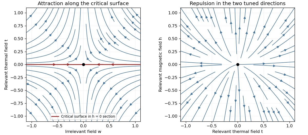
Renormalization-group saddle flow in a zero-field section and two relevant directions transverse to the critical surface
. Details. 
Under the stated homogeneous-scaling assumptions and after fixing irrelevant fields at their limiting values, two relevant scaling fields obey , . These fields are analytic coordinates near the renormalization-group fixed point, proportional to the physical reduced temperature and conjugate field to leading order. The singular free-energy density consequently obeysHere denotes the singular free energy per original site or unit volume, with regular dimensional factors absorbed; the extensive singular part is . Iterate and choose to obtain the scaling hypothesis for critical phenomena:The sign labels the two sides of the transition: describes , the disordered side, while describes , the ordered side. The two functions need not coincide; has the zero-field one-sided derivative appropriate to spontaneous magnetization. The numbers are scaling eigenvalues in logarithmic form: the corresponding discrete RG multipliers are .
The correlation length obeys . The same scale choice gives . Differentiating once and twice with respect to the conjugate field, and twice with respect to temperature, givesAt , instead choose the scale . Then and , so . Thus differentiation and scale matching establishThe first is the Widom scaling relation and the second the hyperscaling relation. The hyperscaling relation requires precisely the regular homogeneous scaling used here. Above the ordinary upper critical dimension, the quartic coupling is dangerously irrelevant in the ordered phase and this derivation cannot discard it: the mean-field critical exponents , do not obey for . At marginal dimensions logarithmic factors likewise require care beyond the displayed pure powers.
There are unlisted articles, also show them or only show them.