
A nearly Hamiltonian system is a weak perturbation of a Hamiltonian system, writtenSince is skew-symmetric, its energy changes by . This identity is exact; it does not require replacing the perturbed trajectory by an unperturbed one.
For a smooth regular family of planar periodic Hamiltonian orbits labeled by energy , the first-order change over one unperturbed period isAssume the family forms a regular annulus, the return section is transverse and , . The return energy then has expansion . Dividing by and applying the implicit function theorem produces a fixed return energy near , hence a nearby periodic orbit for small perturbations.
These planar regular-orbit hypotheses are part of the persistence result. A single averaged energy equation is not automatically sufficient in a higher-dimensional phase space, and a multiple zero requires higher-order terms. Near an infinite-period separatrix, the Melnikov energy-balance method instead measures manifold splitting along a homoclinic orbit or a heteroclinic orbit.
A smooth flow on a smooth manifold is a smooth map withThe identity implies , so each time map is a diffeomorphism. Its generating vector field is ; trajectories solve the autonomous differential equation .
For example, is a smooth flow on the real line, while is a rotation flow on a circle. The second has periodic trajectories, even though the same additive time parameter acts in both examples.
A smooth vector field initially gives only a local flow. The equation has , which blows up at for . On a closed manifold, compactness prevents escape in finite time and local existence can be continued for every real time. Thus every smooth vector field there generates a global smooth flow. On a noncompact manifold, global existence is a separate property.
A hyperbolic toral automorphism is a toral automorphism whose matrix has no eigenvalue on the unit circle. Here , so its determinant is . Invertibility merely over the real numbers would not suffice: multiplication by two on a circle is a many-to-one endomorphism, not an automorphism.
The real stable and unstable subspaces come from the generalized eigenspaces with eigenvalue modulus less than and greater than one. They give the same splitting at every point of the real torus. A Jordan block can add a polynomial factor to the powers of its eigenvalue; choosing a slightly weaker exponential rate absorbs that factor into a constant. Thus contraction forward on the stable subspace and backward on the unstable subspace is uniform over the whole torus, proving that the map is an Anosov diffeomorphism.
For the cat map, has eigenvalues . One is inside and the other outside the unit circle, and their product is one. The toral automorphism mixing criterion applies as well, since a root of unity would lie on that circle.
An Anosov diffeomorphism is a continuously differentiable diffeomorphism of a compact smooth manifold with an invariant splitting of its tangent bundle into stable and unstable vector subbundles satisfying the displayed uniform exponential estimates for , with . Hyperbolic toral automorphisms give examples. An Anosov flow has a further one-dimensional invariant bundle along the flow direction; its definition is a distinct continuous-time version of uniform hyperbolicity.
For an equilibrium point , a homoclinic orbit is a nonconstant trajectory withAt a hyperbolic equilibrium point, the trajectory leaves a neighborhood of along its unstable manifold and returns along its stable manifold. It never reaches in finite time when local solution uniqueness holds. Its closure includes the equilibrium and can form a loop-shaped separatrix.
A completely explicit example iswith Hamiltonian function . Its derivative is zero along every trajectory, and the origin is a saddle point with eigenvalues . The curvelies on . Differentiating gives and , while the hyperbolic secant tends to zero at both time infinities. Thus it is a homoclinic orbit. Changing both signs gives the second loop.
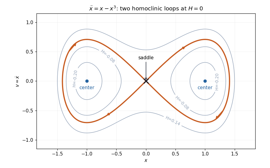
Two exact homoclinic orbits of the double-well oscillator return to the same saddle at infinite time
. Details. 
Each loop bounds periodic orbits around one potential minimum. This is an integrable Hamiltonian system, so a homoclinic loop by itself does not establish chaos. A Shilnikov bifurcation and a simple-zero Melnikov energy-balance method calculation require additional dimensional, spectral or forcing hypotheses.
Coexistence of two stable long-time states at fixed parameters. Initial conditions and sufficiently strong perturbations can select different basins of attraction, allowing a dynamical system to retain a state-dependent memory.
Multistability is coexistence of several stable long-term behaviors at the same fixed parameter values. Those behaviors can be equilibrium points, periodic orbits or more complicated attractors. Different basins of attraction select which behavior a trajectory reaches from its initial state.
For example, has attracting equilibria at and a repelling equilibrium at zero. A sufficiently large perturbation can move a state from one basin to the other, leaving a persistent change after the perturbation ends. This gives a simple mechanism for dynamical memory without changing the governing parameters. Bistability is the two-state case. Hysteresis additionally describes history-dependent switching under a changed control parameter; coexistence alone does not specify a complete hysteresis loop or its switching thresholds.
A Lyapunov exponent is the asymptotic exponential growth rate of an infinitesimal tangent displacement along a dynamical system. For a differentiable flow map, a starting point and a nonzero tangent vector , one convention iswhen the limit exists. A discrete dynamical system uses the derivative of the th iterate and divides by instead. The rate can depend on the point and the direction.
For the linear ordinary differential equation , an eigenvector with real eigenvalue evolves as , so its exponent is . Nonreal eigenvalues contribute their real parts to the growth rate. A polynomial factor from a Jordan block does not change the exponent because .
In a smooth velocity field, the tangent displacement obeys . Its instantaneous stretching rate depends on both the current Jacobian matrix and the current direction. Those can change along the trajectory, so averaging instantaneous largest eigenvalues need not give the actual largest Lyapunov exponent.
The infinitesimal qualification matters. Two trajectories at a fixed finite separation cannot grow apart exponentially forever inside a bounded region: their distance is bounded by the region's diameter. A positive tangent exponent instead concerns the derivative obtained by sending the initial perturbation to zero first. Finite errors follow the linear prediction only until they become large enough that nonlinear effects matter. Likewise, growth rates of moments of a random separation need not equal the exponent along a typical trajectory.
A reflection-symmetric planar cubic model can be expressed in polar variables , , as and . A nonzero equilibrium therefore has , . Adding their squares gives . Each positive root determines an antipodal equilibrium pair. The determinant of the polar linearization there is and its trace is . These formulas distinguish folds of nonzero equilibria from symmetry-forced bifurcations at .
Pattern formation is the development of spatial structure in a system. A common mechanism is the loss of stability of a uniform state to disturbances at a preferred nonzero wavenumber. In Rayleigh-Bénard convection, heating a fluid layer from below can destabilize the conducting state and produce organized convection rolls. In a reaction-diffusion equation, reaction and transport can instead select a spatial concentration pattern.
A linear calculation separates the possible scales. Write a small disturbance as a Fourier mode . Positive real part of means that mode initially grows, and the fastest growing wavenumbers often set the first visible scale. The Swift–Hohenberg equation has , so at small positive it amplifies a band near .
Linear growth is only the onset calculation. A growing disturbance eventually becomes large enough for nonlinear terms to matter. Coupled amplitude equations can then describe competition between modes: one mode can suppress another, several can coexist, or the state can drift or oscillate. The resulting planform includes both the selected wavevectors and their relative amplitudes and phases.
A slowly varying phase modulation describes changes in a pattern's local position and orientation without immediately destroying its periodic structure. Its stability can differ from the stability of a uniform amplitude, as illustrated by the zigzag instability of parallel rolls.
The imperfect soft Duffing-van der Pol oscillatorcombines a softening restoring force, velocity-dependent damping and the symmetry-breaking term . The equilibrium points are and , whenever the latter are real. The associated Jacobian matrix has trace and determinant .
At , the equilibrium equation has the reflection symmetry . For , the branch near zero crosses the zero branch at , giving the generic transcritical bifurcation when . The two nonzero roots meet at , , giving a generic saddle-node bifurcation when . The excluded trace-zero cases have an additional linear degeneracy and require further analysis.
The mechanical energyhas the exact derivative . Thus the sign of energy input can change with displacement even at a fixed value of .
For , the two outer equilibria are saddle equilibria. Their potential barriers are generally unequal when , so a symmetric saddle connection can split into distinct directed connections under an imperfection. The weak-damping heteroclinic splitting of a tilted quartic oscillator calculates their leading parameter curves. Local equilibrium formulas alone do not guarantee a limit cycle or determine its global termination.
An integer matrix with determinant defines a toral automorphismon the real torus . Integer entries make the map independent of the chosen representative. The inverse matrix also has integer entries, so the transformation is invertible. It preserves normalized Haar measure.
The map is a mixing measure-preserving transformation exactly when no eigenvalue of is a root of unity. This can be proved with characters of a real torus , since . Orthogonality givesIf no eigenvalue is a root of unity, a nonzero integer frequency cannot repeat: a repetition would give for some . It therefore eventually leaves every finite set of frequencies. The displayed correlations prove mixing first for trigonometric polynomials, then for square-integrable functions by approximation.
Conversely, a root-of-unity eigenvalue makes singular for some . As an integer matrix it has a nonzero rational kernel vector, which can be scaled to a nonzero integer vector . The nonconstant character is then invariant under , obstructing mixing. The cat map is a mixing example, while the identity matrix gives an invertible measure-preserving map that is not mixing.
Thermodynamic formalism studies weighted trajectories through partition functions, topological pressure and invariant measures. A symbolic potential assigns an orbit segment the weight , where is its accumulated potential. Summing these weights gives ; the limiting logarithmic normalization per step is the pressure.
A one-symbol example shows the mechanism. On a two-symbol full shift, let and . ThenNormalizing gives independent symbol probabilities and . The associated Gibbs measure is therefore an orbit-weight law, not a uniform choice unless .
The same construction can encode geometry. A geometric potential of an expanding map records inverse-branch contraction, while the Feigenbaum geometric potential encodes lengths in a nested partition. Their pressure functions organize spatial scaling and dimension calculations. In that second example, the partition depth is a geometric scale index and should not automatically be identified with elapsed orbit time.
This explains both the usefulness and the limitation of the statistical-mechanics analogy: changing the potential changes which trajectories or geometric pieces receive weight. An arbitrary Gibbs measure need not be absolutely continuous, even when its underlying interval map is expanding.
A piecewise differentiable interval map is uniformly expanding when a constant bounds the derivative on every smooth branch:With a finite partition into monotone branches, a point's itinerary records which branch contains each iterate. A length- cylinder consists of points with the same first branch labels. Wherever this composition is smooth, the chain rule gives .
The mean value theorem then bounds the diameter of a cylinder by the length of the original interval times . Inverse branches therefore determine starting points with exponentially improving spatial precision as more itinerary symbols are specified.
For the doubling map on , the two branches have slope two and the level- cylinders are half-open intervals of length . Their labels are the first digits of the binary expansion. Endpoint conventions matter for unique coding, but not for the cylinder-length estimate.
Expansion describes the map's geometry. A symbolic potential separately specifies statistical weights, so expansion alone does not make every Gibbs measure absolutely continuous. The geometric potential of an expanding map uses the inverse derivative to select weights adapted to interval length.
The Feigenbaum period-doubling map is the universal, even, quadratic-critical fixed map associated with repeated period-doubling bifurcations. One normalization isComposing twice and rescaling therefore reproduces the same graph. This self-similarity is the mechanism behind a common spatial scaling in otherwise different one-dimensional maps with a quadratic maximum.[ref]
Quantitative Universality for a Class of Nonlinear Transformations by Mitchell Feigenbaum. 1978: universal spatial scaling and the period-doubling functional equation
The quadratic maximum means and . Twice applying the chain rule at zero givesThe term involving vanishes, and cancellation is legitimate because the maximum is nondegenerate. Thus the endpoint derivative is determined by the spatial scaling.
Writing makes the successive central intervals shrink by the factor . Their iterates generate the Feigenbaum attractor; nonuniform interval lengths are encoded by the Feigenbaum geometric potential. The constant here describes spatial scaling, rather than the spacing of successive bifurcation parameter values.
The Lorenz system is the three-variable autonomous differential equationIt arose as a low-dimensional model of thermal convection. Edward Norton Lorenz used its numerical solutions in 1963 to study nonperiodic motion and sensitivity to the initial condition, with consequences for long-range weather forecasting.[ref]
Deterministic Nonperiodic Flow by Edward Norton Lorenz. Journal of the Atmospheric Sciences 20 (1963), pages 130–141: convection model, numerical nonperiodic solutions and forecasting implications
The equilibrium points follow directly from the equations. For and , the first gives and the third gives . The second then becomes . Thus the origin always exists, while for there are two additional equilibriawith matching signs in the first two coordinates. The symmetry exchanges them.
The Equilibrium bifurcations of the Lorenz system determine how their stability changes. The separate instantaneous Lorenz error growth at a zero-y crossing calculation concerns a perturbation at one instant; it should not be confused with the long-term Lyapunov exponent.
Evolution is deterministic when a specified initial condition and evolution rule select a unique future orbit. For a discrete dynamical system, applying the same map to the same state gives the same next state. For an ordinary differential equation, uniqueness of the initial value problem is required; merely writing a differential equation does not guarantee it.
Determinism permits both asymptotic stability and sensitive dependence on initial conditions. It does not by itself imply reliable prediction from approximate measurements, and sensitivity does not introduce a random choice into the evolution rule.
For an integrable relaxation modulus, a small constant shear rate sustained from the remote past gives stress equal to that rate times the displayed integral, including any instantaneous solvent mass. For the linear Oldroyd-B model it is . A nondecaying elastic modulus would make this integral infinite rather than describe a fluid with finite steady viscosity.
A control policy selects admissible actions using only the information available at each time, possibly with randomization. General policies may depend on the whole observed history. Nonanticipation and measurability are part of admissibility in a controlled Markov process.
An average-reward optimal policy maximizes long-run expected reward per time step. In a finite recurrent Markov chain, a stationary policy's gain is its expected one-step reward under the stationary distribution. Initial-state effects are encoded by a bias function rather than by the gain. In a communicating finite control problem, the average-reward Bellman equation certifies a policy that is optimal from every initial state.
There are unlisted articles, also show them or only show them.