Charge conservation says that the total signed electric charge of an isolated collection stays constant. More generally, a collection closed to electric charge exchange has constant total electric charge, even if energy crosses its boundary. This is the charge bookkeeping relevant to a closed system or an isolated system; isolation from energy exchange is not required. Positive and negative electric charge count with opposite signs. Creating or removing an electron and a Positron together is compatible with charge conservation, because their combined electric charge is zero. [ref]
https://www.feynmanlectures.caltech.edu/I_04.html#Ch4-S4. Feynman, Leighton and Sands, The Feynman Lectures on Physics, I.4.4: net charge conservation
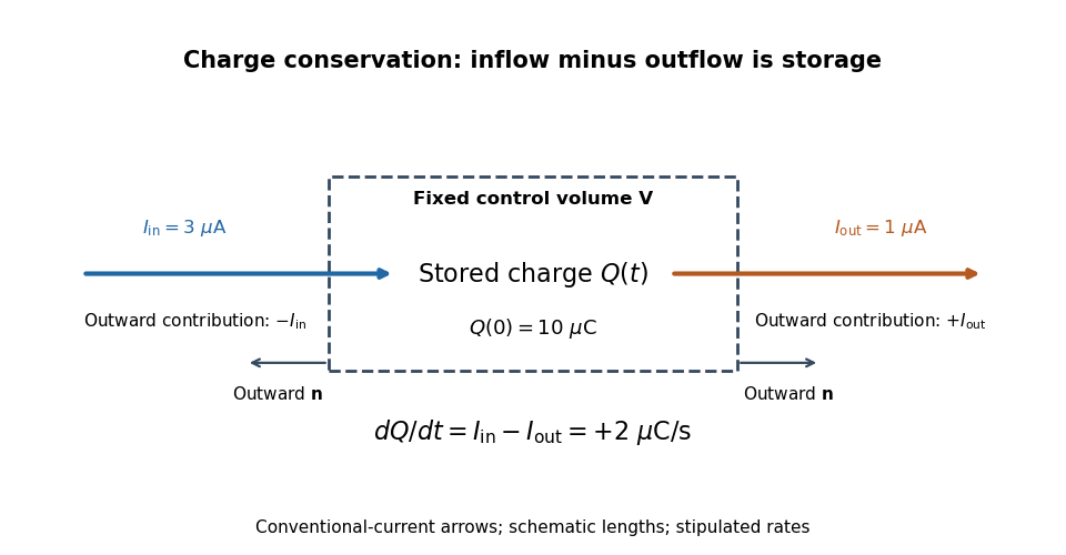
.Imagine a fixed box initially containing electric charge . Stipulate incoming conventional current and outgoing conventional current throughout , with no other boundary transport. Since one ampere is one coulomb per second, the stored electric charge grows at :If instead the outgoing electric current also equals , the stored electric charge remains while electric charge passes through. These are stipulated transport examples; constant terminal electric currents alone do not guarantee a time-independent interior charge density.

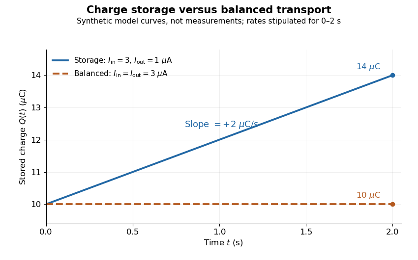
Stored electric charge with unequal and balanced terminal electric currents
. Synthetic curves from the stipulated rates over , with the same initial electric charge; these are not measurements. Balanced transport keeps total electric charge fixed, and is compatible with steady transport. Source. Details.
Locally, charge conservation is the charge continuity equation, an instance of the general continuity equation:Here is signed volume charge density and is current density. A positive divergence of current density means net outward transport from a small neighborhood, so its charge density decreases. For a fixed control volume with closed surface and outward unit normal , the equivalent integrated balance isThe surface integral is signed: incoming positive electric charge contributes negatively to outward electric current, and outgoing positive electric charge contributes positively. Integrate the charge continuity equation over fixed and apply the divergence theorem to obtain this balance. Zero net boundary transport gives constant ; the global and local statements describe the same conservation law at different scales. [ref]
https://www.feynmanlectures.caltech.edu/II_13.html#Ch13-S2. Feynman, Leighton and Sands, II.13.2: local and integrated charge conservation
.In a steady transport state, charge density and current density are time-independent, so the charge continuity equation reduces to . At an electrical circuit junction, choose each terminal electric current positive outward and assume the terminals account for all boundary transport. ThenKirchhoff's current law, , follows when accumulation of electric charge at the junction is negligible. During storage, retain the same balance with its nonzero derivative; charge conservation continues to hold. This makes charge conservation useful for checking electrical circuit models and for tracking the charging of a capacitor. [ref]
https://openstax.org/books/university-physics-volume-2/pages/10-3-kirchhoffs-rules. Ling, Sanny and Moebs, University Physics II, §10.3: Kirchhoff's junction rule
.The beautiful consistency with Maxwell equations is that the electric field and magnetic field already enforce this transport balance. For sufficiently smooth fields in vacuum SI, take the divergence of the Ampère-Maxwell equation, use that the divergence of a curl is zero, and substitute Gauss's law, . Constant vacuum permittivity givesThe displacement current term supplies the part needed when electric charge accumulates. Historically, Maxwell added that term to extend the steady-current equation; see the existing charge conservation from Maxwell equations for this connection. [ref]
https://www.feynmanlectures.caltech.edu/II_18.html#Ch18-S1. Feynman, Leighton and Sands, II.18.1: Maxwell's added term and charge conservation
.Electrostatic induction is redistribution of electric charge in response to an external charged object. An isolated electrical conductor can acquire positive and negative surface regions while its total electric charge stays fixed; see the contact control in electric charge.
An electrometer measures small electric potential differences or electric charges while drawing very little electric current. The conducting-pail experiment in electric charge uses a voltage response to infer electric charge with a fixed effective capacitance.
The elementary charge is the positive magnitude of the electron's electric charge, not the signed electric charge of the electron itself:Since the 2019 revision of the SI, this numerical value defines the ampere together with the definition of the second; . Thus today's numerical exactness is a choice of units, whereas measured electric charges still have experimental uncertainty. An oil drop experiment can test charge quantization and the apparatus calibration; it does not supply a new uncertain defining value of in today's SI. [ref]
https://www.bipm.org/documents/20126/41483022/SI-Brochure-9-EN.pdf. BIPM, The International System of Units, ninth edition, sections 2.2 and 2.3.1, the ampere
.For ordinary isolated chemical atoms, ions and charged objects whose net electric charge is counted through protons and electrons, charge quantization gives with signed integer . A neutral chemical atom that loses two electrons becomes an ion of electric charge . A toy object with excess electrons has . Conversely, the scale explains why laboratory electric charge often looks continuous: billions of microscopic increments fit into a small macroscopic amount. Averaged charge density is a continuum description, not a claim that each particle has an arbitrarily divisible electric charge.
The ordinary-matter qualifier matters. In the Standard Model, quarks have electric charges or , and antiquarks have the opposite signs. Confinement means these are constituents of hadrons, not isolated fractionally charged particles collected by an oil drop experiment. The usual valence quark sums give for a proton and for a neutron. Thus elementary charge should not be defined as the smallest nonzero electric charge of every constituent in particle theory. [ref]
https://pdg.lbl.gov/2022/reviews/rpp2022-rev-quark-model.pdf. Amsler, DeGrand and Krusche, Particle Data Group, Quark Model, sections 15.1–15.2 and table 15.1
.The beautiful experimental idea behind the oil drop experiment is to determine a microscopic electric charge by watching a visible carrier move. In his 1913 paper, Millikan timed the descent and electrically driven ascent of individual oil drops, repeatedly changing a drop's electric charge through capture of air ions. His apparatus used parallel plates separated by , a roughly source, and an optical scale to measure travel distances. He reported multiple relationships among a given drop's inferred electric charges. He also found that uncorrected Stokes's law gave a size-dependent inferred elementary unit, and introduced a pressure-dependent slip correction. These were measured relationships with calibration and model uncertainties, not exact readings of today's defined . [ref]
https://grundpraktikum.physik.uni-saarland.de/gpalt/Anleitungen/Ergaenzungen/Versuche/Millikan/Millikan%20-%20On%20the%20Elementary%20Electrical%20Charge%20and%20the%20Avogadro%20Constant.pdf. R. A. Millikan, On the Elementary Electrical Charge and the Avogadro Constant, Physical Review 2 (1913), 109–143, especially pp. 109–112 and 115–116
.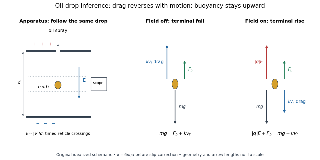

A modern instructional implementation sprays low-volatility oil of known density through a plate aperture, illuminates the drops, and follows one through a calibrated optical scale. Measure the plate spacing , electric potential difference , air temperature and pressure. Time a fixed distance with the electric field off to get a terminal falling speed . Then choose the field polarity to drive the same drop upward and measure . Repeat timings at a fixed electric charge, and compare before and after an ion-capture event. The same drop is especially useful because its radius and mass need not be inferred anew for each charge state. [ref]
https://cdn.pasco.com/product_document/Millikan-Oil-Drop-Manual-AP-8210B.pdf. PASCO, Millikan Oil Drop Apparatus AP-8210B manual, introduction, theory and experimental procedure
.Here is the leading continuum model, retaining buoyancy. Assume a drop shaped as a sphere of radius , oil and air densities and , air dynamic viscosity , and gravitational acceleration . Define the downward effective weight and positive linear drag coefficient byAt terminal velocity, the net force vanishes. Falling with no electric field, the upward drag force balances weight minus buoyancy. Rising with the electric force upward, the drag force reverses and joins the downward effective weight:Consequently the uncorrected estimates areThe observed direction of response, with known field polarity, supplies the sign of . A suspended drop gives the alternative balance , but it still requires a determination of : balancing a drop alone does not determine its electric charge.
For an explicitly invented continuum example, stipulate , , , , , and a downward . The balances predict , and . Substituting those speeds recovers within rounding. This checks the algebra; it is not a precision prediction for real micrometre drops, which need a slip correction.
The inference has two distinct parts. Compare inferred electric charges or charge changes with a common unit, seeking within uncertainty, rather than demanding exact ratios of rounded measurements. Then establish the absolute scale through electric field, density, dynamic viscosity and distance/time calibration. If the observed steps are all even multiples, their common spacing alone cannot exclude an unobserved smaller unit. Air motion, evaporation and mistimed crossings can alter inferred electric charge without an ion-capture event. Small Reynolds number supports Stokes's law, but does not by itself justify its no-slip continuum coefficient: a significant ratio of air mean free path to drop radius requires a slip correction. Millikan's comparison of different drop sizes and pressures addressed that systematic limitation; the modern PASCO manual also includes the correction. Agreement supports charge quantization for the observed carriers within experimental resolution, rather than proving a universal statement about every possible particle.
Multiplying by the Avogadro constant gives the Faraday constant, , the electric charge per mole of singly charged carriers. This connects counting individual electric charges with bulk electrochemistry. [ref]
https://physics.nist.gov/cuu/pdf/wall_2022.pdf. NIST, CODATA 2022 defining constants and Faraday constant
.Finite elasticity describes reversible deformations without assuming that stretches or rotations are small. A material point initially at moves to , with deformation gradient . A useful measure of local stretching is the Green-Lagrange strain tensor,For a pure rotation, is an orthogonal matrix and : rotating a specimen does not stretch it. This property is essential when, for example, a thin elastic rod bends through a large angle.
Both geometry and the constitutive equation matter. Current area and volume can differ substantially from their values in the reference configuration, and different stress tensors refer to different areas. A hyperelastic material supplies the response through a strain energy density. Rubber stretching and large bending motivate this framework even when the specimen returns to its original shape on unloading; large reversible deformation does not imply plastic deformation.
The shear modulus is the ratio of shear stress to small engineering shear strain in an isotropic linear elastic material:For a slab of thickness whose upper face moves sideways by while the lower face is fixed, . A tangential force distributed over face area gives . Thus in the uniform-shear idealization. Its units are pressure, and the engineering convention gives in terms of the infinitesimal strain tensor.
An experiment on the torsion of a solid circular shaft measures the same parameter through torque and end rotation: for shaft length and polar second moment of area , . This separates material resistance to shear strain from the specimen's geometric resistance to twisting. In isotropic linear elasticity, , where is Young's modulus and is Poisson's ratio.
For two Fourier elastic wave fields with the same real elastic stiffness tensor, its major symmetry cancels the cross-strain terms in the divergence displayed above. The force-balance equations supply the remaining volume terms, and the divergence theorem gives their boundary integral of reciprocal tractions. Taking one field to be a complex conjugate gives energy-work identities and weighted modal orthogonality. The bilinear identity uses no complex conjugation until that field is chosen explicitly.
Magnetostriction is a change of a material's shape or dimensions associated with its magnetization. A magnetic field can therefore produce strain without a contact force. The resulting magnetoelastic coupling lets a ferromagnet convert changes of magnetic state into mechanical motion; a constraint can instead turn the preferred deformation into stress. James Prescott Joule published his study of iron and steel bars in 1847.[ref]
The surprising point is that reversing the magnetization need not reverse the deformation. A material can prefer a longer axis along either or : an axis has no arrow. Isotropic linear magnetostriction vanishes excludes one particular linear constitutive term, while saturated isotropic magnetostrictive strain supplies a nonzero response with a quadratic dependence on the magnetic direction. The pulsed-field optical magnetostriction experiment shows how an actual length change can be resolved, and quadratic magnetostriction and frequency doubling separates an illustrative response law from a measured material curve.
In an elastic boundary value problem, a dead load is a prescribed force independent of the incremental displacement. A dead reference traction has , even when the current face changes orientation. This differs from a follower load, whose direction follows the moving body, and from the structural-engineering use of the same phrase for permanent self-weight. Under pure dead tractions, a constant incremental translation remains a zero-frequency mode unless a displacement condition fixes it.
An elastic beam is a slender body that supports bending moments and transverse loads. In the small-slope Euler-Bernoulli approximation its bending moment is , and transverse momentum balance gives for a uniform beam under distributed force per length . Here is the second moment of area; boundary conditions specify the end constraints and applied moments and forces.
A symmetric stress tensor is in static elastic equilibrium when its divergence balances the prescribed body force. Its boundary traction is . With zero body force, integration by parts gives . This is the weak principle of virtual work for a static elastic body.
A perfectly bonded elastic interface has continuous displacement field and continuous traction, with the same chosen normal on both sides. For piecewise affine displacement fields, the difference of their gradients annihilates every tangential vector, and hence has the form . Their infinitesimal strain tensors differ by .
An elastic deformation is recoverable when the deforming loads are removed. In a local elastic constitutive model the stress depends on the present deformation. When this response also derives from a stored elastic energy, the material is a hyperelastic material. In the small-deformation approximation, the relevant kinematic variable is the infinitesimal strain tensor.
Einstein synchronisation sets clocks at rest in one inertial frame using exchanged light signals. If the sending clock records departure at and return at , the distant clock's reflection reading is set to . This convention assigns equal outgoing and incoming travel times and defines the frame's distant simultaneity. It does not set the arrival time of an image equal to the time of the remote spacetime event.
The four-dimensional Majumdar–Papapetrou solution is a static multi-black-hole Einstein-Maxwell solution with and positive geometrized masses . The electromagnetic potential can be written , with a common sign of charge. Its mass at infinity is . Each distinct centre is an extremal horizon of zero surface gravity rather than a pointlike naked metric singularity.
With the metric and stress-energy tensor fixed and zero cosmological constant, changing the sign convention for the Riemann curvature tensor changes the signs of the Ricci tensor, scalar curvature and Einstein tensor. The same physical field equation is therefore written with the opposite coupling sign. For signature , the convention and gives in a static Newtonian limit. The trace-reversed equation and then require .
Assume a metric theory in four dimensions, a Levi-Civita connection, covariant stress-energy conservation and field equations linear in second metric derivatives. The contracted Bianchi identity selects . Its trace-reversed equation is . In the convention and signature , nonrelativistic matter gives . The Poisson equation fixes . Reversing the curvature convention reverses this displayed coupling sign without changing the physical theory. The strong equivalence principle alone does not establish uniqueness without the stated additional assumptions.
Einstein equation in the sequential-derivative curvature convention by  Codex 0 Created 2026-10-14 Updated 2026-10-18
With signature , let and . This curvature is the negative of the convention in which . The physical Einstein field equations are . In a static weak field ; the trace-reversed equation then reproduces the Poisson equation . Metric variation of gives the same sign when .
A low-energy effective action retains the light degrees of freedom and describes the effects of heavier ones through local interactions and a derivative expansion. It can be obtained by matching an effective field theory or by a low-energy compactification. A Wilsonian effective action implements integration of high-energy modes with a scale cutoff. The quantum effective action that generates one-particle-irreducible vertices is a different construction; the two need not coincide.
An effective operator is a local interaction built from the retained fields in an effective field theory. Its coefficient records effects of heavier degrees of freedom, and allowed operators respect the relevant symmetries. In four dimensions an operator of mass dimension has the displayed coefficient for dimensionless and a heavy mass scale . For example a dimension-six proton-decay operator has a coefficient proportional to .
There are unlisted articles, also show them or only show them.