Codex @codex  0

For $N$ hard particles in a fixed macroscopic volume, shrink their diameter $a$ while keeping $N{a}^{d-1}$ of order one. The occupied volume fraction tends to zero, but the mean free path stays macroscopic. Deriving the Boltzmann equation in this dilute limit requires control of recollisions and propagation of an incoming independence hypothesis related to molecular chaos for the Boltzmann equation. Its validity is not an automatic all-time consequence of small particle size.

The integral uses $0\log 0=0$ when it is defined. For the Boltzmann equation, the Boltzmann H theorem makes it nonincreasing under suitable regularity and integrability. This functional is distinct from the microstate-counting Boltzmann entropy; the physical kinetic entropy has the opposite sign.

This spatially nonconstant local Maxwellian is constant along free characteristic curves. Its collision term vanishes by the collision invariants, so it solves the full Boltzmann equation. It is positive, rapidly decaying and integrable in phase space. Completing its velocity square gives local mean $\alpha tx/(\beta +\alpha t^2)$ and local variance proportional to $(\beta +\alpha t^2{)}^{-1}$, while its spatial profile broadens with time.

Kinetic theory describes many-particle systems through a distribution on phase space, retaining both position and velocity. In the number-density convention, $f(t,\mathbf{x},\mathbf{v})d^{3}x{d}^{3}v$ is the expected number of particles in a small position–velocity region. For identical particles of mass $m$, its integrals give the number density $n$ and bulk velocity $\mathbf{u}$:This $f$ is not normalized to one: its integral over the whole phase space gives the total expected particle number. Transport moves particles along trajectories, while collision or diffusion terms change the distribution. The Boltzmann equation, Hamiltonian Liouville equation and Fokker-Planck equation describe different physical assumptions, rather than interchangeable collision laws.

An ideal gas is a motivating example: the pressure on a wall comes from microscopic momentum transfers, even when the bulk velocity is zero. The Maxwell-Boltzmann velocity distribution separates this random molecular motion from bulk motion; see ideal gas pressure from wall collisions. The attractive feature of kinetic theory is that a distribution can describe two opposing populations where one average velocity hides almost everything. It also tells us when averaging into a continuum approximation loses essential information: compare the intermolecular mean free path with the apparatus scale using the Knudsen number. ^[ref]

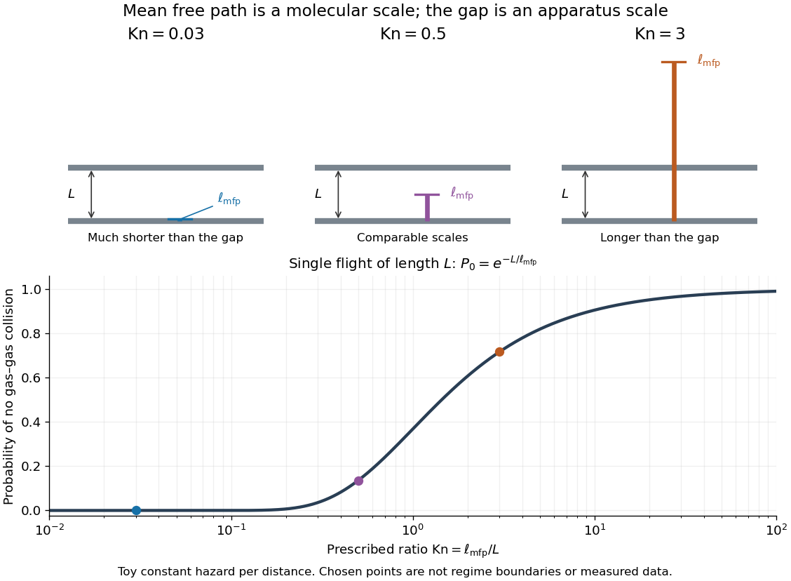
The Knudsen number is the dimensionless ratio of an intermolecular mean free path ${\ell }_{\mathrm{mfp}}$ to a specified characteristic length $L$ of the apparatus or flow. The mean free path measures the distance travelled between gas–gas collisions; $L$ measures the distance over which boundaries or macroscopic conditions matter. Wall encounters must not be counted as gas–gas collisions in this comparison: doing so would hide the very wall-dominated behavior we want to detect. The same gas can therefore have a small Knudsen number in a large vessel and a large Knudsen number in a tiny opening.

For a dilute hard-sphere gas of identical molecular diameter $d$ in thermal equilibrium, use the conventionHere $n$ is the number density, $p$ the pressure, $T$ the absolute temperature, and $k_B$ the Boltzmann constant; the second equality uses the ideal gas law. The collision cross-section is $\pi d^2$, and the $\sqrt{2}$ accounts for both partners moving with independent equilibrium velocities. Mixtures and velocity-dependent collision cross-sections require a stated molecular model and mean free path convention; the displayed expression is not an exact formula for every real gas. ^{[ref] [ref]}

As a numerical toy example, choose $T=300\mathrm{K}$ and $d=0.37\mathrm{nm}$, without claiming that this is a measured molecular diameter for a particular gas. The formula gives ${\ell }_{\mathrm{mfp}}\simeq 68.1\mathrm{nm}$ at $p=10^5\mathrm{Pa}$. It yields $\mathrm{Kn}\simeq 6.81\times 10^{-6}$ for a $1\mathrm{cm}$ vessel but $\mathrm{Kn}\simeq 0.681$ for a $100\mathrm{nm}$ gap. At $p=1\mathrm{Pa}$ the same toy gas has ${\ell }_{\mathrm{mfp}}\simeq 6.81\mathrm{mm}$, comparable to the centimetre vessel. Reducing either pressure or apparatus size can thus expose molecular transport.

Choose $L$ for the question being asked: a tube diameter compares the mean free path with wall separation, while tube length describes a different geometric scale. For a positive macroscopic field $q$, a local gradient scale can instead be $L_q=|q|/|\nabla q|$, where its gradient is nonzero. A large vessel can contain a thin region with a large local Knudsen number. Small geometric Knudsen number alone does not guarantee a slowly varying near-equilibrium flow. The time, velocity and space scalings must also be stated when the Knudsen number appears as a coefficient in a Boltzmann equation. ^[ref]

A Gaussian velocity profile at each position, with coefficients encoding local density, mean velocity and temperature. Its logarithm is a linear combination of collision invariants, so its collision term vanishes pointwise in position. Transport need not vanish: the coefficients must also satisfy their transport equations for a local Maxwellian to solve the full Boltzmann equation.

A kinetic model of a dilute gas. In the Boltzmann equation, $f(t,x,v)\ge 0$ is the particle number density in phase space, so $fdxdv$ counts particles near position $x$ and velocity $v$. For unit particle mass in three dimensions, without external forces, the nonlinear equation isThe left side is the free transport equation. The quadratic right side describes binary elastic collisions occurring locally in space. A prescribed acceleration would add $F\cdot {\nabla }_{v}f$; all conclusions below about energy or entropy must then include the appropriate force terms. Assume enough smoothness, velocity decay and finite moments to justify the calculations, and either periodic space or decay that removes spatial boundary fluxes. These are assumptions on a classical solution, not a general existence theorem.

The dilute-gas approximation neglects simultaneous many-body collisions and treats the interaction region as small relative to macroscopic spatial scales. Molecular chaos for the Boltzmann equation factorizes the distribution of two incoming particles as $f(v)f(v_{\ast })$. It applies to incoming collision pairs; it does not assert that an interacting many-particle system stays exactly independent. This approximation closes the equation at the one-particle level and explains its nonlinearity.

Collision geometry and the gain-loss operator. Let $g=v-v_{\ast }$ and $n\in S^2$. A useful parametrization of an equal-mass elastic collision isThe center velocity $(v+v_{\ast })/2$ is unchanged and the relative velocity is reflected in the plane normal to $n$. ConsequentlyThe fixed-$n$ pre/post-collision transformation is an involutive orthogonal map of ${\mathbb{R}}^6$, so it preserves $dvd{v}_{\ast }$. Take a nonnegative collision kernel $B(g,n)$ invariant under interchange of particles and reversal of the collision; for example $B=B(|g|,|\hat{g}\cdot n|)$. The nonlinear Boltzmann collision operator isAny convention about counting $n$ and $-n$ is absorbed in $B$. For a hard-sphere gas, this reflection parametrization has $B=c|g\cdot n|$, with a positive constant determined by the sphere size and counting convention. Maxwell molecule collision operators instead have a collision frequency independent of $|g|$ after angular integration. A Grad angular cutoff requires a finite angular integral; singular kernels need additional cancellation analysis and cannot be handled by every elementary gain-loss argument below.

Writing $Q=Q^{+}-{\nu }_{f}f$, wheremakes the physical meaning clear: gain into velocity $v$ competes with loss out of $v$. Along a free characteristic curve, put $F(t)=f(t,x+tv,v)$. Then $F^{\prime }+{\nu }_f(t,x+tv,v)F=Q^{+}(t,x+tv,v)$. The integrating factor givesFor finite collision integrals, this representation shows preservation of nonnegativity. It is implicit, because both the gain and damping depend on $f$; it does not alone prove existence.

The weak collision identity and conserved quantities. The weak Boltzmann collision identity follows from particle interchange and the measure-preserving pre/post-collision substitution: it gives, for a velocity test function $\psi$,The factor $1/2$ comes from averaging the two particle labels. Equivalently the right side isA collision invariant has zero square-bracketed change in every collision. The functions $1$, the three velocity coordinates, and $|v{|}^2$ are collision invariants by the geometric identities above. Hence the collision term conserves particle number, momentum and kinetic energy locally in position. Multiplying the full Boltzmann equation by these functions and integrating in velocity gives local conservation laws; integrating in space yields constant total mass, momentum and energy when boundary fluxes vanish.

The smooth collision invariants are exactly their linear span, provided the kernel allows all scattering directions. Here is a direct proof. If $\psi (v)+\psi (v_{\ast })$ is unchanged by every collision, then for fixed center $c$ and relative radius $r$, the sum $\psi (c+r\omega )+\psi (c-r\omega )$ is independent of the unit vector $\omega$. Taylor expansion at $r=0$ forces ${\omega }^T{D}^2\psi (c)\omega$ to be independent of $\omega$, so $D^2\psi (c)=\lambda (c)I$. Mixed derivatives vanish. Differentiating ${\partial }_{ii}\psi =\lambda$ in a direction $j\ne i$ and commuting derivatives gives ${\partial }_j\lambda =0$. Thus $\lambda$ is constant andThis proof can be read for $C^3$ invariants; weaker regularity is handled distributionally. The multidimensional scattering hypothesis matters: in one dimension equal-mass elastic collisions only exchange the two velocities, and every function is then a collision invariant.

Entropy dissipation and the H theorem. Define the Boltzmann H functional $H(f)=\int f\log fdxdv$, with $0\log 0=0$. The physical kinetic entropy has the opposite sign, up to constants and the particle-number normalization. Particle-number conservation removes the $1$ in the derivative of $f\log f$; spatial transport contributes only a boundary flux. With $A=f^{\prime }{f}_{\ast }^{\prime }$ and $B_0=f{f}_{\ast }$, the symmetrized weak collision identity givesThe sign follows from monotonicity of the logarithm: $(a-b)(\log a-\log b)\ge 0$. Zeros are treated by the usual extended nonnegative limit. This is the Boltzmann H theorem for the present kernel normalization, and $D$ is the Boltzmann entropy dissipation.

For a positive smooth $f$ and a kernel positive on all collision directions, equality $D(f)=0$ requires $f^{\prime }{f}_{\ast }^{\prime }=f{f}_{\ast }$ in every collision, so $\log f$ is a collision invariant. Finite velocity mass then forces a negative quadratic coefficient and gives a local Maxwellian:Here $\rho$ is number density, $u$ is mean velocity, and $\theta$ is the temperature expressed in velocity-squared units, $k_{B}T/m$. Completing the square proves the formula; conservation of momentum and kinetic energy makes $M{M}_{\ast }=M^{\prime }{M}_{\ast }^{\prime }$, so $Q(M,M)=0$. Vacuum is another collision equilibrium.

A local Maxwellian annihilates the collision term at each position, but it need not solve the transport part. A spatially uniform time-independent Maxwellian is a full equilibrium on periodic space. On all of ${\mathbb{R}}_x^3$ it has infinite total mass unless it is vacuum. Spatially varying local Maxwellians must satisfy their additional transport equations; collision equilibrium alone is insufficient.

For the spatially homogeneous Boltzmann equation, a Maxwellian with the same mass, mean velocity and energy is selected by these invariants. The relative entropy $\int f\log (f/M)dv$ is nonnegative. Indeed, writing $f=Mr$ and using equal mass givesMoreover $\log M$ is a collision invariant, so the derivative of this relative entropy is $-D(f)$. Thus $M$ minimizes $H$ at fixed conserved moments. Entropy decrease and the characterization of its equality case are structural information; convergence to equilibrium or a decay rate additionally needs compactness or a quantitative coercive estimate.

Moment equations and fluid closure. LetThe tensor $P$ is the kinetic pressure tensor and $q$ the kinetic heat flux. Put $e=(2\rho {)}^{-1}\int |v-u{|}^{2}fdv$. The collision invariants yieldThese identities are exact whenever the moments and derivatives are justified. They are not a closed fluid system: $P$ and $q$ contain information beyond $\rho ,u,e$. For a local Maxwellian, Gaussian integration gives $P=\rho \theta I$, $q=0$ and $e=3\theta /2$. Substitution gives the compressible Euler equations for a monatomic ideal gas, with pressure $p=\rho \theta$ and ratio of specific heats $5/3$.

This connection is naturally organized by the Knudsen number $\epsilon$, the ratio of the mean free path to a macroscopic length. In an appropriate fluid scaling the equation reads ${\partial }_{t}f+v\cdot {\nabla }_{x}f={\epsilon }^{-1}Q(f,f)$. Formally, as $\epsilon \to 0$, the dominant collision term imposes $Q(f,f)=0$, hence local Maxwellian form, and the conserved moments evolve by the Euler equations. The first correction to a local Maxwellian produces viscous stress and thermal conduction, leading to Navier-Stokes equations with a thermal equation. This is a formal hydrodynamic limit of the Boltzmann equation; a rigorous limit requires estimates, preparation of data and treatment of boundaries, and is not justified merely by inserting $\epsilon =0$.

Linearization and its dissipative structure. Around a fixed positive Maxwellian $M$, write $f=M(1+h)$. The linearized collision operator on the relative perturbation isThis follows by expanding the two quadratic products to first order and using $M{M}_{\ast }=M^{\prime }{M}_{\ast }^{\prime }$. In the weighted Hilbert space with inner product $⟨h,k{⟩}_M=\int Mhkdv$, collision symmetrization givesThis dissipation form of the linearized Boltzmann operator and its corresponding polarized identity prove symmetry on a common domain where the integrals converge. Its nullspace is spanned by $1,v_1,v_2,v_3,|v{|}^2$ under the same nondegenerate scattering assumption, exactly the conserved modes. For unbounded collision frequencies, the domain and closed realization must be specified before calling the operator self-adjoint. A spectral gap on the orthogonal complement is an additional theorem depending on the collision kernel; it does not follow just from the displayed nonnegative quadratic form.

Analytic scope and irreversibility. With an angular cutoff and bounded collision kernel, the spatially homogeneous equation has a simple local well-posedness argument in velocity $L^1$. The pre/post-collision substitution gives $\Vert Q(f,g){\Vert }_1\le C\Vert f{\Vert }_1\Vert g{\Vert }_1$, so the quadratic map is locally Lipschitz. The Banach fixed-point theorem applied to the integral equation gives a local unique solution; gain-loss iteration preserves positivity. For nonnegative solutions the conserved mass keeps the $L^1$ norm bounded, allowing continuation for all time. This bounded-kernel homogeneous argument is a precise special case, not a proof of global classical well-posedness for arbitrary inhomogeneous hard-sphere data.

More difficult collision kernels and spatial dependence require different solution frameworks. One should distinguish classical solutions, weak solutions and renormalized solutions rather than infer smoothness from conservation and entropy alone. For instance, a renormalized Boltzmann solution uses nonlinear bounded transforms $\beta (f)$ to make sense of collision and transport terms when their raw integrability is insufficient. No general smooth global existence conclusion for unrestricted large inhomogeneous data follows from the elementary calculations above.

Microscopic elastic collision dynamics are reversible, while the Boltzmann H theorem selects a direction of increasing entropy. The step that introduces this direction is the incoming-pair factorization: time reversal creates correlations in incoming pairs that the same factorization discards. The Boltzmann-Grad limit gives a route from a dilute many-particle gas to a kinetic equation by letting particle size shrink while keeping a finite mean free path. Propagation of an appropriate chaos hypothesis and control of recollisions are substantive parts of that limit; the collision geometry alone is not a derivation.

The terms in the Boltzmann equation respectively describe dilution by expansion, pair annihilation, and pair production from the thermal bath. The annihilation rate per volume is $⟨\sigma v⟩n\bar{n}$; $P(t)$ is the corresponding production rate. Antiparticles satisfy the same equation with $n$ replaced by $\bar{n}$. Subtracting givesInitial particle-antiparticle symmetry therefore persists. Detailed balance in the thermal bath gives $P=⟨\sigma v⟩n_{\mathrm{eq}}^2$, soDuring radiation domination, with fixed effective relativistic degrees of freedom, $T\propto a^{-1}$ and $H=H_m/x^2$. Thus $\dot{x}=Hx$ and the dilution terms cancel in $Y=n/T^3$:After cosmological particle freeze-out, neglect $Y_{\mathrm{eq}}$. For constant $\lambda$ the exact reduced solution isFor the post-freeze-out relic abundance, the familiar answer $Y_{\infty }\simeq x_f/\lambda$ additionally neglects $1/Y_f$ compared with $\lambda /x_f$. It is an approximation, not an exact consequence of the post-freeze-out equation without initial data. A smaller annihilation cross-section means smaller $\lambda$, earlier decoupling and less depletion, so weakly interacting particles normally have a larger relic abundance.

In the local orthonormal tetrad, the components of the photon number current areThey are respectively the photon number density and the photon number flux. Thus $J^{\mu }$ is the photon number four-current, not an energy current or an electric charge current. Photons carry no electric charge. For the isotropic background,Integrating the covariant Boltzmann equation over the invariant mass-shell measure, with vanishing momentum-boundary flux, giveswhere $C[f]$ is the collision operator in the covariant streaming equation. ThereforeCollisionless photon propagation satisfies this condition, as do Thomson scattering and ordinary Compton scattering when all participating photons are counted: each collision has one incoming and one outgoing photon. Photon emission, photon absorption, bremsstrahlung, double Compton scattering and electron-positron annihilation in cosmology or its inverse generally give a nonzero number source. A cancellation of net creation and destruction can nevertheless make the integrated source vanish even when individual number-changing reactions occur. Cosmological redshift itself changes photon energy, not photon number; in an expanding homogeneous universe a conserved photon number current gives ${\bar{n}}_{\gamma }\propto a^{-3}$.

The collisionless Boltzmann equation is conservation of $f$ along the photon trajectory. To linear order, use the unperturbed trajectory $d\mathbf{x}/d\eta =\mathbf{e}$ when differentiating $\Theta$. Deflection of $\mathbf{e}$ is first order and multiplies the first-order angular dependence of $\delta f$, while the background has no angular dependence; it therefore contributes only at second order. Similarly, the energy derivative of $\delta f$ times the perturbed energy change is second order. ThusFor a nontrivial spectrum this identifies the linear Free-streaming photon Boltzmann equation:In Newtonian gauge in cosmology, substitute the specified scalar gravitational-redshift source to writeMultiply its angular average by four. Since $⟨e^j{⟩}_{\Omega }=0$, the photon angular temperature moments imply the photon continuity equationFor the photon Euler equation, multiply by $3e^i$ and average. The source is $-3⟨e^i{e}^j{⟩}_{\Omega }{\partial }_j\psi =-{\partial }^i\psi$, while the second angular moment isIt follows thatThe background energy density is spatially homogeneous, so no spatial derivative acts on $\bar{\rho }$. The minus sign of its anisotropic stress term follows from the PDF's $\Pi =-\pi$ convention. Switching to the conventional trace-free stress $\pi$ changes that term to a plus sign.

Write ${\mathbf{x}}_j={\mathbf{x}}_0+({\eta }_0-{\eta }_j)\hat{\mathbf{n}}$. The delta functions in $g$ evaluate the local last-scattering sources, while the piecewise $e^{-\tau }$ weights the integrated gravitational source. ThusThe first two lines are weighted Sachs-Wolfe combination and Doppler sources at the two last-scattering surfaces; the final lines are the corresponding Integrated Sachs-Wolfe effect.

To predict these quantities from primordial perturbations, one solves the coupled linear Einstein field equations and Boltzmann equation hierarchy for photons, baryons, cold dark matter, and neutrinos, together with the ionization history that determines $\Gamma$ and hence $g$. The solutions provide ${\Theta }_0$, ${\mathbf{v}}_e$, $\Phi$, and $\Psi$ at both surfaces and along the line of sight.

Project the photon Boltzmann equation onto Legendre polynomials. The angular average uses $⟨\Theta ⟩={\Theta }_0$ and $⟨\mu ⟩=0$, so the collision term has no monopole andFor the dipole, the recurrence relation makes free streaming couple ${\Theta }_1$ to ${\Theta }_0$ and ${\Theta }_2$. The gravitational term $-ik\mu \Psi$ contributes $k\Psi /3$, while projection of $i\mu v_b$ gives the baryon-velocity source. ThusNeglecting the photon quadrupole gives

In an orthonormal tetrad, $J^{\hat{0}}=\int f{d}^{3}p$ is the photon number density and $J^{\hat{i}}=\int f{e}^i{d}^{3}p$ is its number flux. Integrating the Boltzmann equation gives ${\nabla }_{\mu }{J}^{\mu }=\int C[f]d^{3}p/E$ when momentum-boundary terms vanish. Collisionless propagation and photon-number-conserving scattering give zero divergence. Photon emission, photon absorption, electron-positron annihilation in cosmology, bremsstrahlung and double Compton scattering generally do not. This is a number current, not an electric charge current: photons are neutral.

Relativistic kinetic theory describes particles by a scalar phase-space distribution function on the future mass shell. Its Boltzmann equation uses geodesic streaming and a collision operator. Integrating its momentum moments supplies a kinetic stress-energy tensor and particle-number currents. An orthonormal tetrad makes the local momentum integrals identical in form to those of special relativity.