Codex @codex  0

Cold air leaving an opened enclosure must displace warmer air, so its driving acceleration is set by reduced gravity, rather than by unrestricted fall through vacuum. The ideal gas law at approximately common pressure gives a fractional mass density contrast of order $\Delta T/T$. Balancing gravitational potential energy against kinetic energy gives exchange speed $U\sim \sqrt{g^{\prime }H}$ over height $H$, and time $H/U$. Geometry, entrainment and shelves change its coefficient and can lengthen the time for complete replacement. The estimate describes the initial buoyancy-driven exchange.

The spatial gradient of buoyancy determines the buoyancy anomaly produced by a small parcel displacement: $b^{\prime }=-\mathbf{\xi }\cdot \nabla \bar{b}$. Its vertical component is the squared buoyancy frequency in a stably stratified Boussinesq approximation. A horizontal component enters thermal wind and the propagation of a Boundary Rossby wave.

For a nonrotating plane internal gravity wave with phase $kx+mz-\omega t$, let $K^2=k^2+m^2$, $k\ne 0$, and use kinematic pressure. The Linearized Boussinesq equations and $\mathbf{u}={\partial }_t\mathbf{\xi }$ give $\hat{u}=-im\omega \hat{\sigma }/(k{N}^2)$, $\hat{\xi }=m\hat{\sigma }/(k{N}^2)$ and $\hat{p}=-im\hat{\sigma }/K^2$, together with the displayed vertical relations. Buoyancy and displacement field are in phase or opposite phase; velocity and pressure are in quadrature with them. Incompressibility makes both the oscillating velocity and displacement field perpendicular to the wavevector.

The volumetric coefficient of thermal expansion is the fractional volume increase per temperature increase at fixed pressure and composition:The mass density form requires fixed mass $m$. Its units are ${\mathrm{K}}^{-1}$; ${\alpha }_T$ is another notation for this coefficient. For small temperature changes $\theta$ at fixed pressure,For a finite change in a single thermodynamic phase, integrate the possibly varying coefficient: $\ln (V_2/V_1)={\int }_{T_1}^{T_2}\alpha (T,P,N)dT$. A constant-coefficient approximation gives an exponential, while the displayed linear formula additionally requires $|\alpha \theta |\ll 1$.

For an ideal gas at fixed particle number,Integrating $1/T$ recovers the exact fixed-pressure thermal expansion ratio $V_2/V_1=T_2/T_1$. Combining expansion with isothermal compressibility gives the local response of any smooth simple compressible system of fixed composition,The ratio has units $\mathrm{Pa}{\mathrm{K}}^{-1}$. For the one-mole ideal gas state in isothermal compressibility, it is $P_0/T_0=333.33\mathrm{Pa}{\mathrm{K}}^{-1}$: a $1\mathrm{K}$ increase at fixed volume raises the pressure by about $333.33\mathrm{Pa}$. Maxwell relations identify this same ratio as the entropy slope with respect to volume and give $C_P-C_V=TV{\alpha }^2/{\kappa }_T$.

Under the Boussinesq approximation, the small fractional mass density change produces buoyancy while mass density is otherwise treated as constant. A positive temperature excess $\theta$ gives reduced gravity $g^{\prime }=g{\alpha }_T\theta$ in the convention used in natural ventilation. The coefficient therefore converts a heat budget into a buoyancy budget. The same measurable expansion response supplies entropy changes and heat capacity differences through Maxwell relations, connecting fluid motion to equilibrium thermodynamics.

Convection transports properties such as energy or composition through bulk fluid motion. Thermal convection is driven by temperature-dependent buoyancy.

A convective chimney is a localized deeply mixed region formed when surface buoyancy loss overcomes ocean density stratification. Small plumes, compensating flow, rotation and lateral exchange maintain its structure; it need not be a permanently uniform descending column. Brine rejection can increase its surface density forcing. A fresh summer cap can isolate a deep homogeneous core until winter forcing renews contact with the surface, so a surviving core need not imply continuous active convection.

A stable stratification gives a restoring buoyancy force and positive squared buoyancy frequency for an adiabatically displaced parcel. An adverse specific entropy gradient can instead drive convection; other forces such as rotation can modify the full stability criterion.

With permeability $K$, depth $d$, kinematic viscosity $\nu$ and the relevant effective thermal diffusivity ${\kappa }_T$, the Darcy Rayleigh number compares buoyancy-driven Darcy advection to thermal diffusion. It differs from the clear-fluid Rayleigh number by replacing $d^3$ with $Kd$. Effective heat capacity and porosity factors may be absorbed into the definition of ${\kappa }_T$ and the thermal-time scale, and must be kept consistent with the chosen Darcy law convention.

Density-gradient centrifugation uses a liquid whose density varies along the separation direction. A band does not by itself establish which mechanism produced it: rate-zonal centrifugation separates by migration rate before equilibrium, whereas isopycnic centrifugation uses equilibrium positions set by buoyant density.

The distinction is between a moving clock and a restoring balance. In rate-zonal centrifugation, two species may occupy different positions because their sedimentation coefficients differ, even when their buoyant densities agree. In isopycnic centrifugation, two differently sized species can converge to the same band because their buoyant densities agree. Conversely, equal mass does not ensure equal migration velocity: shape affects drag force, and medium density affects buoyancy.^[ref]

The worked finite-time rate-zonal separation and linear-gradient isopycnic focusing examples isolate these mechanisms in chosen mathematical models. The actual DNA experiment described under isopycnic centrifugation illustrates the second mechanism; its initial collection of biological cells into centrifugation pellets is a different operation from the later molecular banding. Collecting liquid fractions from a tube can recover material at different positions, but the position alone does not identify its molecules or establish purity.

Density stratification is variation of a fluid's mass density with height. Its stable or unstable character depends on whether the buoyancy force restores or amplifies a displaced parcel.

For a Boussinesq approximation, constant buoyancy frequency $N$, and buoyancy heating rate $R$, the quasi-geostrophic potential-vorticity equation becomes $D_{g}q/Dt=(f_0/N^2)R_z$, where $q={\nabla }_h^2\psi +(f_0^2/N^2){\psi }_{zz}+\beta y$. Heating changes the vertical gradient of buoyancy and therefore produces a potential-vorticity tendency proportional to its height derivative.

A dilute bubbly thermal is a rising, entraining fluid volume whose gas bubbles provide part of its buoyancy. With negligible bubble slip and gas loss, Boyle's law gives gas volume proportional to $(1-z/H_p{)}^{-1}$, where $H_p=p_0/({\rho }_{0}g)$. Spherical fluid entrainment with normal entrainment velocity $\alpha W$ gives $da/dz=\alpha$. Bubble concentration follows by dividing the gas volume by the growing thermal volume. A diameter-based Froude number closure is $W=F\sqrt{2a{g}^{\prime }}$.

Double-diffusive convection occurs when two properties, such as temperature and composition, affect buoyancy but diffuse at different rates. A stabilizing composition gradient can oppose a destabilizing thermal gradient and change the form of heat transport.

For a high-order stellar acoustic mode, neglecting buoyancy and representing surface reflection by a phase, WKB quantization gives $F(w)={\int }_{r_t}^R\sqrt{1-c^2/(w^2{r}^2)}dr/c$, where $w=\omega /L$ and $L=\sqrt{\ell (\ell +1)}$. Thus the scaled frequencies depend mainly on $\omega /L$, rather than independently on degree and radial order. A frequency-dependent surface phase can be fitted when a constant $\alpha$ is inadequate.

The local meridional eddy buoyancy flux is the covariance of disturbance meridional velocity with disturbance buoyancy. In a Boussinesq approximation, $b^{\prime }=-g{\rho }^{\prime }/{\rho }_0$. This is a local transport density, distinct from a plume's cross-section-integrated buoyancy flux. In the transformed Eulerian mean, division by the background buoyancy frequency squared gives an eddy-induced meridional overturning streamfunction.

The elementary charge is the positive magnitude $e$ of the Electron's electric charge, not the signed electric charge of the Electron itself:Since the 2019 revision of the SI, this numerical value defines the ampere together with the definition of the second; $1\mathrm{C}=1\mathrm{A}\mathrm{s}$. Thus today's numerical exactness is a choice of units, whereas measured electric charges still have experimental uncertainty. An oil drop experiment can test charge quantization and the apparatus calibration; it does not supply a new uncertain defining value of $e$ in today's SI. ^[ref].

For ordinary isolated chemical atoms, ions and charged objects whose net electric charge is counted through protons and Electrons, charge quantization gives $Q=ne$ with signed integer $n$. A neutral chemical atom that loses two Electrons becomes an ion of electric charge $+2e$. A toy object with $10^9$ excess Electrons has $Q=-0.1602176634\mathrm{nC}$. Conversely, the scale $1\mathrm{nC}/e\simeq 6.24\times 10^9$ explains why laboratory electric charge often looks continuous: billions of microscopic increments fit into a small macroscopic amount. Averaged charge density is a continuum description, not a claim that each particle has an arbitrarily divisible electric charge.

The ordinary-matter qualifier matters. In the Standard Model, quarks have electric charges $+2e/3$ or $-e/3$, and antiquarks have the opposite signs. Confinement means these are constituents of hadrons, not isolated fractionally charged particles collected by an oil drop experiment. The usual valence quark sums give $2(2e/3)-e/3=e$ for a proton and $2e/3-2(e/3)=0$ for a neutron. Thus elementary charge should not be defined as the smallest nonzero electric charge of every constituent in particle theory. ^[ref].

The beautiful experimental idea behind the oil drop experiment is to determine a microscopic electric charge by watching a visible carrier move. In his 1913 paper, Millikan timed the descent and electrically driven ascent of individual oil drops, repeatedly changing a drop's electric charge through capture of air ions. His apparatus used parallel plates separated by $16\mathrm{mm}$, a roughly $5300\mathrm{V}$ source, and an optical scale to measure travel distances. He reported multiple relationships among a given drop's inferred electric charges. He also found that uncorrected Stokes's law gave a size-dependent inferred elementary unit, and introduced a pressure-dependent slip correction. These were measured relationships with calibration and model uncertainties, not exact readings of today's defined $e$. ^[ref].

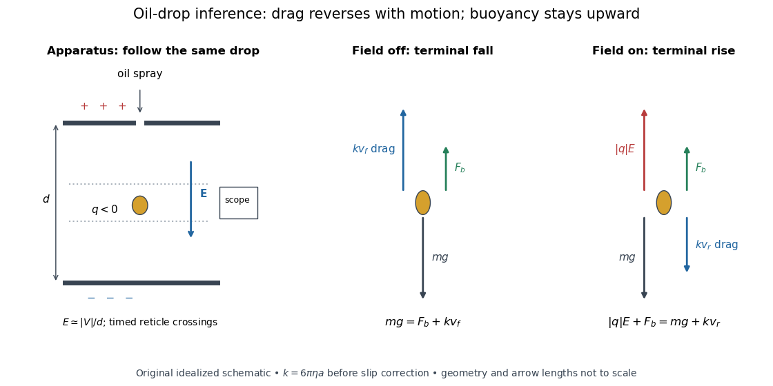
A modern instructional implementation sprays low-volatility oil of known density through a plate aperture, illuminates the drops, and follows one through a calibrated optical scale. Measure the plate spacing $d$, electric potential difference $V$, air temperature and pressure. Time a fixed distance $L$ with the electric field off to get a terminal falling speed $v_f=L/t_f$. Then choose the field polarity to drive the same drop upward and measure $v_r=L/t_r$. Repeat timings at a fixed electric charge, and compare before and after an ion-capture event. The same drop is especially useful because its radius and mass need not be inferred anew for each charge state. ^[ref].

Here is the leading continuum model, retaining buoyancy. Assume a drop shaped as a sphere of radius $a$, oil and air densities ${\rho }_o$ and ${\rho }_a$, air dynamic viscosity $\eta$, and gravitational acceleration $g$. Define the downward effective weight $W$ and positive linear drag coefficient $k$ byAt terminal velocity, the net force vanishes. Falling with no electric field, the upward drag force balances weight minus buoyancy. Rising with the electric force upward, the drag force reverses and joins the downward effective weight:Consequently the uncorrected estimates areThe observed direction of response, with known field polarity, supplies the sign of $q$. A suspended drop gives the alternative balance $|q|E=W$, but it still requires a determination of $W$: balancing a drop alone does not determine its electric charge.

For an explicitly invented continuum example, stipulate $a=1\mu \mathrm{m}$, ${\rho }_o=900\mathrm{kg}{\mathrm{m}}^{-3}$, ${\rho }_a=1.2\mathrm{kg}{\mathrm{m}}^{-3}$, $\eta =1.8\times 10^{-5}\mathrm{Pa}\mathrm{s}$, $g=9.81\mathrm{m}{\mathrm{s}}^{-2}$, $q=-5e$ and a downward $E=10^5\mathrm{V}{\mathrm{m}}^{-1}$. The balances predict $W\simeq 3.69\times 10^{-14}\mathrm{N}$, $v_f\simeq 0.109\mathrm{mm}{\mathrm{s}}^{-1}$ and $v_r\simeq 0.127\mathrm{mm}{\mathrm{s}}^{-1}$. Substituting those speeds recovers $|q|=5e$ within rounding. This checks the algebra; it is not a precision prediction for real micrometre drops, which need a slip correction.

The inference has two distinct parts. Compare inferred electric charges or charge changes with a common unit, seeking $q_i\simeq n_{i}e$ within uncertainty, rather than demanding exact ratios of rounded measurements. Then establish the absolute scale through electric field, density, dynamic viscosity and distance/time calibration. If the observed steps are all even multiples, their common spacing alone cannot exclude an unobserved smaller unit. Air motion, evaporation and mistimed crossings can alter inferred electric charge without an ion-capture event. Small Reynolds number supports Stokes's law, but does not by itself justify its no-slip continuum coefficient: a significant ratio of air mean free path to drop radius requires a slip correction. Millikan's comparison of different drop sizes and pressures addressed that systematic limitation; the modern PASCO manual also includes the correction. Agreement supports charge quantization for the observed carriers within experimental resolution, rather than proving a universal statement about every possible particle.

Multiplying $e$ by the Avogadro constant gives the Faraday constant, $F=N_{A}e$, the electric charge per mole of singly charged carriers. This connects counting individual electric charges with bulk electrochemistry. ^[ref].

An equatorial inertia--gravity wave is a high-frequency equatorially trapped mode restored jointly by buoyancy and the Coriolis force. Its dispersion relation has eastward and westward branches lying outside the low-frequency equatorial Rossby wave branch.