Codex @codex  0

Atomic force microscopy maps surfaces and measures small interactions using a sharp tip attached to a compliant cantilever. In a common modern readout, a laser reflects from the cantilever onto a split photodetector, turning bending into an electrical signal. A scanner moves the tip relative to the sample; feedback can adjust height to maintain a chosen interaction signal. With calibrated stiffness $k$, a small static deflection $\delta$ gives force $F\approx k\delta$. The measured image combines surface geometry, tip geometry and interaction physics, so narrow features can appear broadened. Gerd Binnig, Calvin Quate and Christoph Gerber introduced the instrument in 1986.^[ref] Modern force measurements additionally require calibrated cantilever stiffness.^[ref]

A force-microscopy mode keeping the probe in contact while monitoring cantilever deflection. Constant-deflection feedback records the vertical actuator motion needed to maintain an approximate normal-force setpoint; finite probe geometry and specimen deformation still affect the image.

Measurement of lateral tip–surface forces from torsion of an atomic-force-microscope cantilever.

An instability in a compliant force probe when the attractive force gradient exceeds the restoring stiffness of the cantilever. The tip then jumps from a noncontact branch into contact; the missing branch cannot be followed quasistatically with that stiffness.

A rising force branch means that an already exposed polypeptide segment is being stretched while the remaining structure resists further extraction. At a force peak a structural barrier is crossed; protein denaturation or release of additional chain increases the available polymer contour length, so the force falls at almost the same imposed separation. Stretching then loads the next remaining barrier. The sawtooth pattern therefore reports a sequence of mechanically resistant intermediates, not a regular spring oscillation. The cantilever deflection gives force, while its own deformation must be removed from the imposed separation to infer molecular extension.

A membrane protein also requires work to disrupt membrane anchoring, helix packing and contacts with lipids or neighboring molecules. The retinal-containing interior contributes a bulky, specifically packed scaffold; exposing chain must overcome these steric hindrance as well as hydrogen bond and electrostatic interactions. A force peak need not correspond one-to-one to one complete helix, and its height depends on loading rate and pathway, not just an equilibrium folding Gibbs free energy.

Salt changes electrostatic screening and specific ion binding. Screening can reduce either repulsion or attraction, so “more salt always weakens the protein” is false. The primary study underlying these kinds of traces identifies relatively salt-insensitive steric hindrance around the retinal and additional salt-sensitive barriers. Its interpretation associates some added barriers with screening of destabilizing electrostatic repulsion. The supplied traces likewise show a changed set of intermediate peaks, rather than a uniform rescaling of one curve.^[ref]

Exact assignment of every arrow to a residue requires structural and statistical information beyond one representative trace. No such assignment is inferred here. The printed reference to titin in the following paragraph is inconsistent with the stated specimen and the membrane-protein traces; the physical interpretation here concerns bacteriorhodopsin, while the worm-like-chain expression is a generic polymer approximation.

In spectrin unfolding by force spectroscopy, the cantilever measures tension through its calibrated deflection, while displacement of the pulling point increases the separation of the protein attachments. The protein extension is obtained after allowing for cantilever compliance and any linker extension; it is not simply the commanded displacement.

A folded spectrin repeat stores much of its backbone in a compact domain. Between unfolding events, the already released chain is stretched: increasingly straight conformations have fewer accessible configurations, and the resisting entropic force rises nonlinearly. A peak is reached when a still-folded domain crosses an unfolding barrier on the timescale of the imposed loading. Its released backbone increases the available contour length abruptly. At nearly the same end-to-end distance the fractional extension $x/L$ is then smaller, so tension drops. Pulling resumes on the next, longer-chain elastic branch. Repeated release of domains produces the saw-tooth sequence.

The record is therefore evidence for sequential mechanical unfolding of modular structure, not repeated stretching of a fixed-length rod. For the nominal eight-domain construct, successive branches correspond to increasing numbers of unfolded repeats. The order and rupture forces can fluctuate because barrier crossing is thermally activated and depends on loading rate, structural heterogeneity and pulling geometry; equivalent repeats need not rupture at identical force.

The horizontal separation between worm-like-chain fits at the same force estimates the added contour length, whereas the vertical force drop at one extension reflects redistribution of tension. These are distinct measurements. A repeat increment near the specified $31.7\mathrm{nm}$ is consistent with repeated similar structural units. The gain is a net release relative to the folded span and attachment geometry; $31.7/106\mathrm{nm}$ is not automatically the universal contour length of a peptide residue.

During unloading, relaxation and possible refolding can restore compact domains. Hysteresis would indicate dissipative or kinetically delayed processes. Neither the peak force alone nor an arbitrary saw-tooth area directly equals an equilibrium unfolding free energy: one must separate chain elasticity, cantilever storage, irreversible loss and pulling-rate effects. The worm-like-chain branches describe released-chain elasticity, not the molecular transition state responsible for a rupture peak.

The AFM pulls a tethered molecule through its cantilever. Deflection, multiplied by a calibrated cantilever spring constant, measures force; support motion must be corrected for that deflection and any linker compliance to obtain molecular extension. Initially folded structure can resist extension, then contacts break and more polypeptide polymer contour length becomes available. The readable trace rises with increasing extension, with fluctuations and a strongly rising large-extension part. It should not be interpreted as a direct image of individual amino acids or as establishing a unique microscopic unfolding pathway.

An ideal inextensible freely jointed chain with the stated segment count and length hasIts mean extension is strictly below $14\mathrm{nm}$ at every finite force. Thus the quoted $15\mathrm{nm}$ maximum does not establish ideal FJC behaviour: if both numbers are taken literally, it exceeds the model's polymer contour length by about $7\%$. Finite segment stretch, inaccurate effective segment parameters, additional linkers or an extension-zero/calibration error can account for such a difference. If the numerical descriptions are approximate, the discrepancy may be within their uncertainty; even exact agreement with a polymer contour length would not prove freely jointed statistics. Low-force fluctuations and the full force–extension relation are separate tests.

In a tensile atomic force microscopy measurement, a DNA tether connects the cantilever tip and a surface. Moving the support stretches the molecule, and calibrated cantilever deflection supplies the tensile force; extension must be corrected for cantilever deflection and any linkers. At low force, extension mainly straightens an initially fluctuating coil, giving approximately linear entropic elasticity. At higher force the available conformations become increasingly aligned, so additional extension costs progressively greater force. The readable source curve then continues beyond the nominal inextensible-model contour length, which signals a failure of that simple model or of the stated parameter interpretation, rather than negative elasticity.

Take the clamp at $s=0$ with $x(0)=y(0)=\theta (0)=0$. An end force without an applied end moment gives the free-end condition ${\theta }^{\prime }(1)=0$. With $F=0$, the Euler elastica equation is $EI{\theta }^{\prime \prime }+G\cos \theta =0$. For $|G|/(EI)\ll 1$, $\theta$ is small, so the leading equation isIntegrating with the two boundary conditions givesTo first order, $x^{\prime }=\cos \theta =1+O(G^2)$ and $y^{\prime }=\sin \theta =\theta +O(G^3)$. HenceEquivalently $y(x)=G{x}^2(3-x)/(6EI)$ at leading order, the familiar cantilever response. Because $G<0$, the deflection is downward. The free-end displacement field and slope are $y(1)=G/(3EI)$ and $\theta (1)=G/(2EI)$. The remainder notation holds with fixed positive $EI$ and nondimensional unit rod length.

In scanning tunneling microscopy, $I\propto e^{-2\kappa z}{\int }_{E_F}^{E_F+eV}{\rho }_s(\mathbf{r},E)dE$ under simplified constant-tip-density assumptions, with $\kappa \simeq \sqrt{2m\varphi }/\hslash$. A constant-current height map mixes actual surface height with local electronic density, barrier/work-function changes and tip structure. Changing bias can change contrast without moving atoms. Scanning tunneling spectroscopy instead records energy dependence, often through $dI/dV$; tip states, matrix elements and thermal or modulation broadening still affect its interpretation.

In atomic force microscopy, contrast comes from tip-sample forces or their gradients: short-range chemical bonding and repulsion, dispersion forces, electrostatics and sometimes magnetism or capillary forces. Contact deflection, oscillation amplitude and frequency shift are different observables. A force-gradient image can therefore differ from a geometrical-height image, and changing the tip termination can strongly change atomic contrast.

STM's exponential distance sensitivity can give excellent vertical sensitivity; usable resolution also depends on current noise, feedback, vibration and drift. Lateral contrast depends on the apex orbitals and electronic spatial extent, not merely the nominal tip radius. In AFM, broad-tip geometrical convolution broadens larger features; a sharp terminal atom and short-range forces can produce much finer atomic contrast. Cantilever stiffness, amplitude, frequency noise, force range, thermal fluctuations and feedback influence height sensitivity. In both techniques, detecting a small displacement is distinct from resolving two neighboring objects.

An example is the Cu(111) surface-state standing-wave experiment. Low-temperature STM and spatially resolved spectroscopy connect atomic steps or defects in a surface map with surrounding energy-dependent electronic interference patterns. Their period changes with bias, whereas a fixed structural corrugation would not acquire that electronic dispersion. The result shows why spectroscopic maps reveal surface-electron scattering beyond what a height image alone identifies.^[ref] The apparent fringes are not a second set of equally spaced surface atoms.

Atomic force microscopy senses tip–sample interactions through a compliant cantilever. Contact deflection, oscillation amplitude, phase or resonance frequency can be converted into a feedback signal. Chemical bonding and short-range repulsion, van der Waals forces, electrostatic forces and, where relevant, magnetic or capillary interactions produce contrast. Apparent height at a fixed force or frequency setpoint can therefore contain interaction contrast as well as geometry. Lateral resolution depends on the effective tip apex and interaction range; finite tip radius broadens features. Vertical sensitivity also depends on thermal and detector noise, cantilever calibration, vibration, drift and feedback bandwidth. Strongly localized short-range forces favor atomic resolution, whereas extended interactions average over more of the tip and surface.

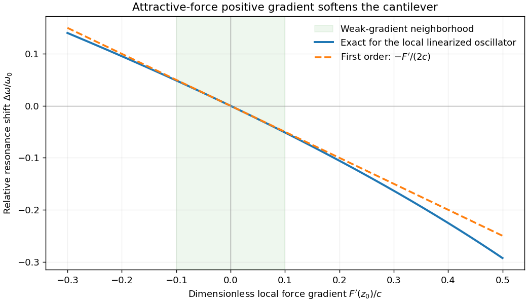
For small oscillations about equilibrium separation $z_0$, write $z=z_0+x$ and linearize $F(z)=F(z_0)+F^{\prime }(z_0)x$. The constant force is absorbed into the equilibrium displacement. The cantilever equation becomesConsequently the small-amplitude AFM frequency shift isThe linear expression is the small-force-gradient approximation, $|F^{\prime }|\ll c$, in addition to the small-oscillation assumption. For an attractive force $F=-C/z^2$, $F^{\prime }>0$ and the resonance softens. A finite oscillation amplitude samples a weighted range of forces rather than only the gradient at one separation, and $F^{\prime }\ge c$ destroys local stability in this simple static model.

In a scanning electron microscope, a focused electron beam scans the surface and a detector records an emitted signal at each beam position. Low-energy secondary electrons escape from near the surface; changes in local slope, edges and detector-facing geometry give strong secondary-electron topographic contrast. Backscattered electrons result from elastic deflection of primary electrons and generally have a larger yield for higher atomic number. Their backscattered-electron atomic-number contrast therefore helps separate compositional regions. Detector geometry, crystal orientation and topography can also affect this signal, so brightness is not a unique elemental identification.

An environmental scanning electron microscope admits gas around the specimen while pressure-limiting apertures and differential pumping preserve the electron-optical column's vacuum. Electron collisions ionize the gas. Positive ions can neutralize negative charging of a poorly conducting specimen, enabling observation without a conductive coating. A gaseous secondary electron detector uses gas amplification to collect secondary-electron signals under these conditions. Gas pressure, path length and scattering must be controlled because they also affect the probe and background.^[ref]

Finally, acquire an energy-dispersive X-ray spectroscopy spectrum at each pixel to add elemental specificity. The beam creates inner-shell vacancies, and characteristic X-rays emitted as they fill identify chemical elements. Selecting fitted characteristic-line intensities yields elemental maps that can be compared with the electron image. Peak overlap, detector response, absorption and the X-ray-generating interaction volume limit identification, quantification and spatial resolution. This gives chemical-element contrast; resolving different bonds or oxidation states generally needs more detailed spectral information than one broad elemental map.

The fixed support supplies the end shear force and the largest bending moment, $FL$. In elementary beam bending, the greatest longitudinal tensile and compressive stresses lie on opposite outer faces of the section at the fixed end, with zero longitudinal bending stress on the neutral axis. For a downward tip load on a horizontal cantilever, the upper face is in tension and the lower face in compression. Transverse shear stress has a different distribution, largest near the neutral axis for a rectangular section; “highest force” should therefore be interpreted with the stress component specified.

With $w$ fixed, bending strength requires $h=\sqrt{6FL/(w{\sigma }_f)}$. Substitution into the cantilever mass givesThe material performance index to maximize is thereforeChanging the free geometric variable changes the strength exponent. A stiffness-limited problem would instead involve Young's modulus; the supplied modulus does not enter this strength-only index.

The rectangular second moment of area is $I=w{h}^3/12$. The maximum bending stress in the cantilever is $FL(h/2)/I=6FL/(w{h}^2)$. If $h$ is fixed, choose the minimum allowed width $w=6FL/({\sigma }_f{h}^2)$. Its mass is thenThus the material performance index to maximize isFor unequal tensile and compressive strengths, use the smaller permissible stress in this symmetric section. The derivation assumes bending-strength control, not a separate deflection, shear, buckling or existing-crack constraint.

Both outer faces of the cantilever are loaded, so use the pine's lower longitudinal compressive strength, $40\mathrm{MPa}$, rather than its $85\mathrm{MPa}$ tensile strength. Consistent SI units give $M_A$ values $(2.564,2.143,0.7273)\times 10^5{\mathrm{m}}^2{\mathrm{s}}^{-2}$ for steel, aluminium and pine respectively. Their $M_B$ values are $5.734,8.748,11.499\mathrm{P}{\mathrm{a}}^{1/2}{\mathrm{m}}^3\mathrm{k}{\mathrm{g}}^{-1}$. Hence Design A: steel best, pine worst; Design B: pine best, steel worst. Aluminium is intermediate in both cases. These rankings concern the stated strength constraint; a toughness or deflection constraint could change feasibility.

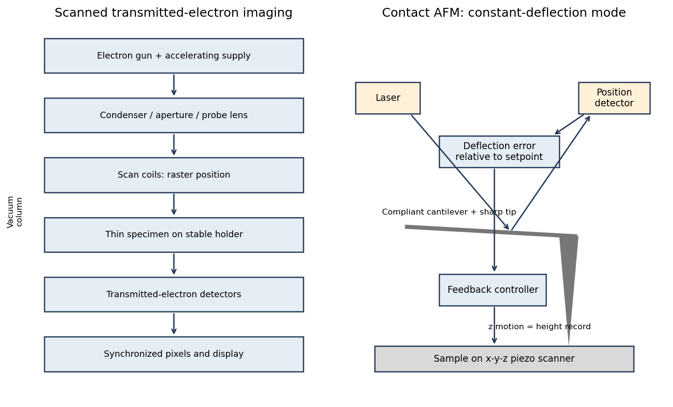
In contact-mode atomic force microscopy, a sharp tip on a compliant cantilever remains in contact with the surface while a feedback loop controls its normal deflection. A laser reflected from the cantilever onto a position-sensitive detector converts bending into an electrical error signal. With calibrated deflection $d$ and stiffness $k_c$, the normal force is approximately $F=k_{c}d$ under the stated contact convention.

A piezoelectric scanner raster-scans the sample or tip. The controller adjusts vertical position to maintain the chosen deflection setpoint; that vertical displacement is recorded as topography. The right panel of the microscopy diagram identifies tip, cantilever, optical deflection readout, controller and vertical actuator.

The result is a probe-accessible surface, affected by finite tip shape, sample deformation, adhesion and feedback bandwidth. Lateral friction can distort or damage a soft surface, so constant deflection is not a guarantee of unchanged specimen structure.

The measured potential is a spatially weighted electrostatic signal, not an infinitesimal-point voltage. The apex, cone and cantilever all contribute capacitance; increasing lift height weakens the signal and broadens its lateral averaging. Small pits can consequently show reduced or distorted contrast.

Imperfect topographic tracking changes the true separation on the lift pass, producing crosstalk correlated with pit geometry. Tip contamination or work-function drift changes the reference. Adsorbed water, mobile charges, illumination, atmosphere and surface states can change the specimen during measurement; semiconductor band bending can also depend on the applied electrical excitation.

There is a tradeoff between small lift height and suppressing short-range/topographic interference. Repeat at several heights, check trace/retrace and an electrical reference, and compare with independently measured electrical response. A stable potential contrast is evidence of a local electrostatic difference, not by itself proof of a particular dislocation's conductivity.

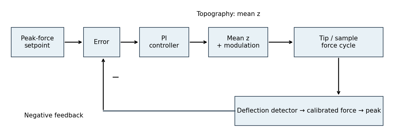
The controlled quantity is the maximum repulsive force in each tapping cycle. In PeakForce quantitative nanomechanical mapping, a vertical modulation below the cantilever resonance produces a force-distance cycle at each pixel. The optical lever measures deflection; the calibrated cantilever stiffness converts this to force. Subtract the measured peak force from the setpoint and use proportional-integral control to adjust the mean vertical scanner position. Excessive peak force makes the controller withdraw the sample or tip; insufficient force makes it approach. The scanner position required to maintain the setpoint supplies the topography signal. This controls the top of the repulsive branch in the preceding curve, rather than the oscillation amplitude used in conventional tapping mode.^[ref]

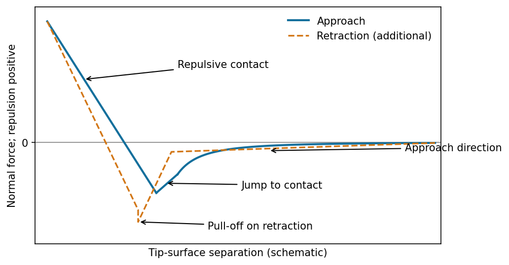
The atomic force microscope measures the cantilever deflection $d$, converted to normal force by $F=k_{c}d$ after calibration. On approach, the force is initially almost zero, then attractive; a sufficiently steep attractive force gradient causes jump-to-contact. After contact, further approach bends the cantilever and indents the sample, giving a rising repulsive branch. With tip-surface separation increasing to the right, approach proceeds from right to left. The instability occurs when the magnitude of the attractive force gradient exceeds the cantilever stiffness. The contact-branch slope depends on both cantilever and sample compliance.

friction force microscopy records cantilever torsion caused by lateral tip–sample force. Choose the detector sign so that friction on a flat region contributes positively during a left-to-right trace. On a common laboratory-position axis, write the two signals schematically asHere $B$ is an offset and $G$ represents a slope-related lateral-force or detector cross-talk contribution. A reversed electronic convention reverses all plotted signs without changing the physical conclusions.

At the same controlled normal contact force $N$, the flat-region contribution is approximately $F_f=\mu N$. The lower perovskite structure plateaux give a larger trace–retrace separation than the upper inorganic surface, because their coefficient of kinetic friction is larger. Genuine friction reverses sign with scan direction, so a larger friction magnitude means a higher positive trace and a more negative retrace in this convention.

Sloped edges produce additional peaks or shoulders. The normal reaction to a slope has a lateral component, and the finite tip flank can contact the rim, so edge contrast is not a direct map of the local friction coefficient. With the two scans registered and load control maintained,The half-difference therefore emphasizes friction while the half-sum diagnoses common geometrical contributions. Real contact mechanics and imperfect registration can prevent exact cancellation. The bottom panel of the figure shows these two kinds of contrast separately.