Codex @codex  0

Use Gaussian elimination with partial pivoting, choosing a largest absolute entry in the uneliminated part of each pivot column. The first pivot is two in row one, with multipliers $1/2,1/2,1/5$ for rows two, three and four. The second-column candidates are then $-1,0,-2/5$, so row two stays as pivot and the remaining nonzero multiplier is $2/5$ for row four. The augmented matrix at this stage isThe third pivot is three, so swap rows three and four. The final multiplier is $-1/4$, leaving last pivot $-2$. Carrying that swap through the previously stored multipliers givesThe transformed right side is $(3,1,0,0{)}^T$. Back substitution gives $z=0$, $y=0$, $x=-1$ and $w=1$, hence $\boxed{(w,x,y,z)=(1,-1,0,0)}$.

For the eigenvalue claim, put $S=P^{T}L$. It is invertible because a permutation matrix and a unit lower triangular matrix are invertible. The factorization gives $A=SU$, soSimilar matrices have the same characteristic polynomial and therefore the same eigenvalues with algebraic multiplicities. This proves the claim without changing the prescribed elimination method.

A QR decomposition is a factorization $A=QR$ with $Q^{T}Q=I$ and $R$ upper triangular. An orthogonal transformation preserves the Euclidean norm becauseFor the basic QR algorithm, start with $A_0=A$ and repeatedly formIn a convergent diagonal form, the diagonal entries give the eigenvalues; practical symmetric-matrix implementations use shifts and deflation to obtain and isolate such convergence. The basic unshifted iteration alone need not converge diagonally for every symmetric input.

At every step, however,Thus each iterate is orthogonally similar to its predecessor. Similar matrices have the same characteristic polynomial and eigenvalues, including multiplicities, so induction proves that every iterate has exactly the original eigenvalues. Orthogonal similarity also preserves symmetry.

The endpoint bounds printed in this part are false. Take $n=3$, $ϵ=1/100$ and $\delta =9/10$, which obey $\delta <(n-1)/2-ϵ=99/100$. The characteristic polynomial isIt has $P(101/100)=-31599/10^6<0$ and $P(5/4)=441/1600>0$, so it has a real root strictly between $1.01$ and $1.25$, outside the first printed interval. There is a unique eigenvalue in the transpose's isolated first disc of radius $1/4$, identifying it as the first eigenvalue. Similarly $P(301/100)=-40999/10^6<0$ and $P(13/4)=41/64>0$ give a root above $3.01$, violating the last printed interval. The approximate three roots are $1.02675615$, $1.94385374$ and $3.02939011$.

There is nevertheless a corrected enclosure proving the claimed reality. Under the stated condition write $R=ϵ+\delta <(n-1)/2$. The large first row disc is disjoint from the large last column disc, since their centres are $n-1$ apart and their radii are both $R$. Every eigenvalue lies both in the row union and in the column union. It cannot belong to both large discs, so it lies in at least one of the fixed small discsThese fixed discs are pairwise disjoint. At $\delta =0$ each contains one eigenvalue. Eigenvalues depend continuously, as a multiset, on the entries; throughout the connected allowed interval no eigenvalue can move between these separated fixed sets while remaining in their union. Thus each still contains one, counted with multiplicity. Complex-conjugate pairing now proves each is real. The valid conclusion isThe source's stronger width $ϵ$ at both endpoints does not persist after adding the corner entry; it was valid for the unperturbed matrix only.

The enclosure method is Complementary row and column Gershgorin isolation.

The known active neutrinos are too light and too fast to supply the dominant cold dark matter. Their relativistic decoupling leaves substantial free streaming, which erases rather than seeds sufficiently small-scale structure; their allowed mass density is also inadequate for the dominant cold component. Changing a light active neutrino from Dirac to Majorana does not remove those problems. What can change the picture is an enlarged neutral-fermion sector containing sterile states with different masses, production and decay rates. A sufficiently long-lived sterile neutrino in a Majorana state can be a dark-matter candidate; Majorana character alone supplies neither stability nor the correct abundance.

For the spinor calculation, put $a=p_z/(E+m)$ and define $A=N(1-a)/2$, $B=N(1+a)/2$. Applying the given chiral projectors givesConsequentlywhere the last equality uses $E^2-p_z^2=m^2$. Same-chirality Lorentz scalar products instead vanish: for example ${\overline{U}}_{1L}{U}_{1L}=0$. The nonzero overlaps demonstrate the Lorentz scalar structures coupling left and right chirality. For $U$ to $U$ this is a particle-number-preserving Dirac coupling; for $U$ to the charge-conjugate $V$ sector it can describe a lepton-number-violating Majorana coupling.

There is a normalization subtlety: both displayed overlaps equal the on-shell mass parameter used to define the spinors. A chiral scalar spinor overlap verifies a coupling structure without fixing an independent Lagrangian coefficient $M_L$. Repeating the on-shell construction with mass parameter $M_L$ would instead give the corresponding overlap $M_L$; this is a different input, rather than a newly derived parameter. The independent coefficients of a Dirac mass term and a Majorana mass term are defined byThe Majorana terms connect a field with its charge conjugate and violate the corresponding continuous lepton phase symmetry by two units. With only unbroken Standard Model gauge symmetry, a left-handed Majorana mass also requires electroweak symmetry breaking or an appropriate higher-dimensional operator; it is not an arbitrary gauge-invariant bare mass for a lepton doublet.

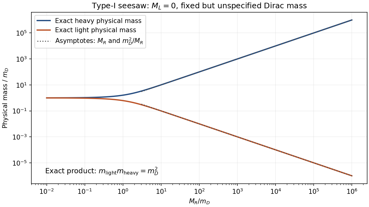
Use an all-left-handed Weyl basis ${\mathbf{n}}_L=({\nu }_L,{\nu }_R^c{)}^T$. For real parameters the one-family Dirac-Majorana mass matrix isWriting $({\nu }_{1L},{\nu }_{2L}{)}^T=\left(\begin{array}{cc}\cos \theta & -\sin \theta \\ \sin \theta & \cos \theta \end{array}\right)({\nu }_L,{\nu }_R^c{)}^T$ gives an orthogonal diagonalization, with $\tan 2\theta =2m/(M_R-M_L)$ up to the rotation-sign convention. Massive-particle chirality and helicity are not identical; the familiar left/right helicity language becomes an approximation in the relativistic regime.

The characteristic polynomial isIts roots areFor Majorana fermions the nonnegative physical masses, as explained by physical Majorana mass and signed eigenvalue, are $|{\lambda }_{\pm }|$ after a possible field rephasing; a negative real eigenvalue is not a negative physical rest mass. When $M_R\gg |m|,|M_L|$,The light state is predominantly ${\nu }_L-(m/M_R){\nu }_R^c$, while the heavy state is predominantly ${\nu }_R^c+(m/M_R){\nu }_L$. Each mass eigenstate combines its Weyl component and charge conjugate to form a Majorana field.

For $M_R=10^{12}\mathrm{GeV}$, the heavy mass is approximately $10^{12}\mathrm{GeV}$. In the type-I limit $M_L\simeq 0$,The seesaw light-mass estimate needs a Dirac scale: no unique numerical light mass follows because the Dirac mass and $M_L$ were not supplied. As an explicitly conditional illustration, choosing $m=100\mathrm{GeV}$ and $M_L=0$ gives $10\mathrm{eV}$; this is an assumed Dirac scale, not additional exam data or a prediction from $M_R$ alone. A heavy seesaw state is also not automatically stable enough to be dark matter.

The conventional minimal Pati-Salam model gauge group isThe group printed in this paper is different: it contains two $SU(4)$ factors and only one $SU(2)$. This is a discrepancy in the original PDF, not just in the transcription. The standard-model discussion below uses the conventional intended Pati-Salam model model. A literal theory with the printed product would require additional fermion representations and symmetry-breaking data that are not specified.

The Pati-Salam model unifies the three quark color charges with lepton number as a fourth color charge. A family forms $(4,2,1)$ left-handed and $(4,1,2)$ right-handed multiplets, including a right-handed neutrino. The extended color charge group contains quark-lepton gauge bosons, while the right-handed weak factor supplies right-handed charged currents after symmetry breaking. The Pati-Salam charge embedding isThe original paper explicitly develops the smaller local subgroup $SU(2{)}_L\times SU(2{)}_R\times SU(4{)}_C$, as well as a larger underlying global structure; neither distinction licenses silently replacing the printed group.^[ref] The product group is a quark-lepton unification scheme rather than a simple gauge group with one automatically common coupling. Breaking the right-handed and $B-L$ symmetries can generate a large $M_R$ and light/heavy Majorana neutrinos through the seesaw. The gauge group alone does not uniquely fix their masses or guarantee a dark-matter lifetime.

The most important laboratory test of Majorana character is neutrinoless double beta decay,with no outgoing neutrinos. Under light-neutrino exchange, the amplitude involvesThe coherent squared mixing elements allow phase cancellations. A null result constrains this combination within the assumed mechanism, rather than proving that all neutrinos are Dirac.

The observable is a peak in summed electron energy at the decay Q value, unlike the continuous two-neutrino spectrum. Enriched source material, large exposure, good energy resolution, underground operation and radiopure construction suppress backgrounds. germanium arrays use the source as a semiconductor detector; xenon time-projection chambers combine ionization, light and event-position information; bolometers measure deposited energy through a temperature rise. The GERDA collaboration's Phase-I study is a concrete example of an enriched-germanium source-detector search with background suppression.^[ref] energy calibration, resolution tails, radon and material backgrounds, cosmic-ray vetoes, signal-like event topology and sideband fits all need independent checks before a Q-value excess is convincing. Collider same-sign dilepton processes can test heavier Majorana states, but require a specified production and decay mechanism. Lepton-number violation, absolute-mass measurements and oscillation data provide complementary information; oscillations alone do not settle Majorana character.

The specified energy requires $n_x+n_y=2$, so the relevant energy eigenspace has the orthonormal basisApplying the creation and annihilation operators givesThus its matrix in this ordered basis isWriting $q=\hslash \lambda$, the characteristic polynomial gives $\lambda ({\lambda }^2-4)=0$. The possible angular momentum eigenvalues are thereforeFor completeness, normalized simultaneous energy and angular momentum eigenstates areEach value occurs once in this energy eigenspace. Equivalently, circular ladder operators of a two-dimensional oscillator give $\hat{H}=\hslash \omega ({\hat{N}}_{+}+{\hat{N}}_{-}+1)$ and ${\hat{L}}_z=\hslash ({\hat{N}}_{+}-{\hat{N}}_{-})$. With $N_{+}+N_{-}=2$, the difference can only be $2,0,-2$.

A QR decomposition is $A=QR$, with $Q$ orthogonal and $R$ upper triangular. Orthogonality gives $Q^{\mathsf{T}}Q=I$, and therefore $\Vert Qx{\Vert }^2=x^{\mathsf{T}}{Q}^{\mathsf{T}}Qx=x^{\mathsf{T}}x=\Vert x{\Vert }^2$, proving invariance of the Euclidean norm.

The unshifted QR algorithm starts with $A_0=A$. At step $k$, factor $A_k=Q_k{R}_k$ and set $A_{k+1}=R_k{Q}_k$. ThenThus consecutive matrices are related by orthogonal similarity, so they have the same characteristic polynomial and eigenvalues. Induction proves every iterate has the original eigenvalues. Symmetry is also preserved. When the iteration converges to diagonal form, its diagonal entries are the eigenvalues; practical implementations use shifts and deflation to improve convergence.

Use two plane waves, $|\mathbf{k}⟩$ and $|\mathbf{k}-\mathbf{G}⟩$, as a basis near their Bragg degeneracy. The potential has Fourier coefficients $V_{\pm \mathbf{G}}$; its zero Fourier coefficient vanishes. All other plane waves are off resonance and are neglected in the leading nearly-free electron model. With ${\epsilon }_{\mathbf{k}}={\hslash }^2{k}^2/(2m_e)$, the Schrödinger equation reduces to the Hermitian matrix problemSetting the characteristic polynomial equal to zero givesSolving this quadratic equation givesFor the real cosine potential its coefficient $V_G$ is real; the absolute-value form also allows an arbitrary choice of origin and corresponding Fourier phase.

At the Brillouin-zone boundary, $\mathbf{k}\cdot \mathbf{G}=G^2/2$, the free energies are equal. The two standing waves have different probability densities relative to the lattice potential and are split byRepeating this avoided crossing at the reciprocal lattice boundaries joins smooth branches into energy bands. In one dimension a nonzero Fourier coefficient opens a gap at the corresponding crossing. In higher dimensions a direct gap at one wavevector need not give a common forbidden energy interval at every wavevector: different bands may still overlap in energy. The present two-dimensional example remains metallic even though the crossings are locally gapped.

For the rectangular lattice, choose real-space primitive vectors $a\hat{\mathbf{x}}$ and $b\hat{\mathbf{y}}$. The reciprocal lattice vectors areDefine the half-widths of the first Brillouin zone by $K=\pi /a$ and $L=\pi /b$. Their values and the zone areA primitive reciprocal cell can be drawn with a corner at the origin; its centred translate is the first Brillouin zone here. Its area is $4{\pi }^2/(ab)=37.9600\mathrm{n}{\mathrm{m}}^{-2}$.

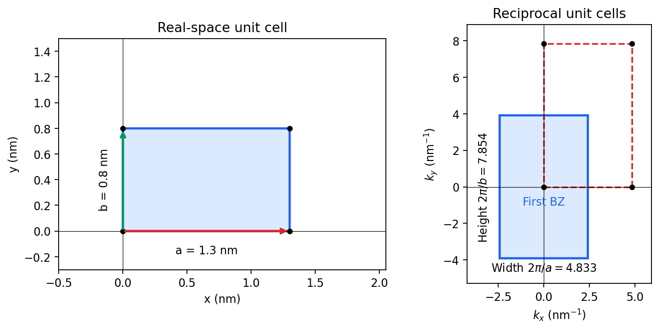
Including both spin states, counting the occupied free-electron states per unit area givesConsequentlyThe occupied disk has precisely the area of the first Brillouin zone, but their shapes differ: $K<k_F<L$. It protrudes through both vertical zone boundaries and does not reach the horizontal ones. Thus two electrons per cell do not imply a filled first band in the absence of a separating band gap.

Fold the protruding caps by $\pm {\mathbf{G}}_x$. The original circle and the translated circle intersect at $k_x=K$, $k_y=\pm \sqrt{k_F^2-K^2}$. The potential mixes these states and replaces each crossing by an avoided crossing. The lower branch reconnects into two open sheets running across successive zones in the $k_x$ direction; the upper branch forms a closed lens-shaped pocket about a vertical zone boundary. In a reduced-zone sketch its two halves sit at opposite edges, but periodic identification makes them one closed sheet. This is rectangular-lattice Fermi-surface reconstruction.

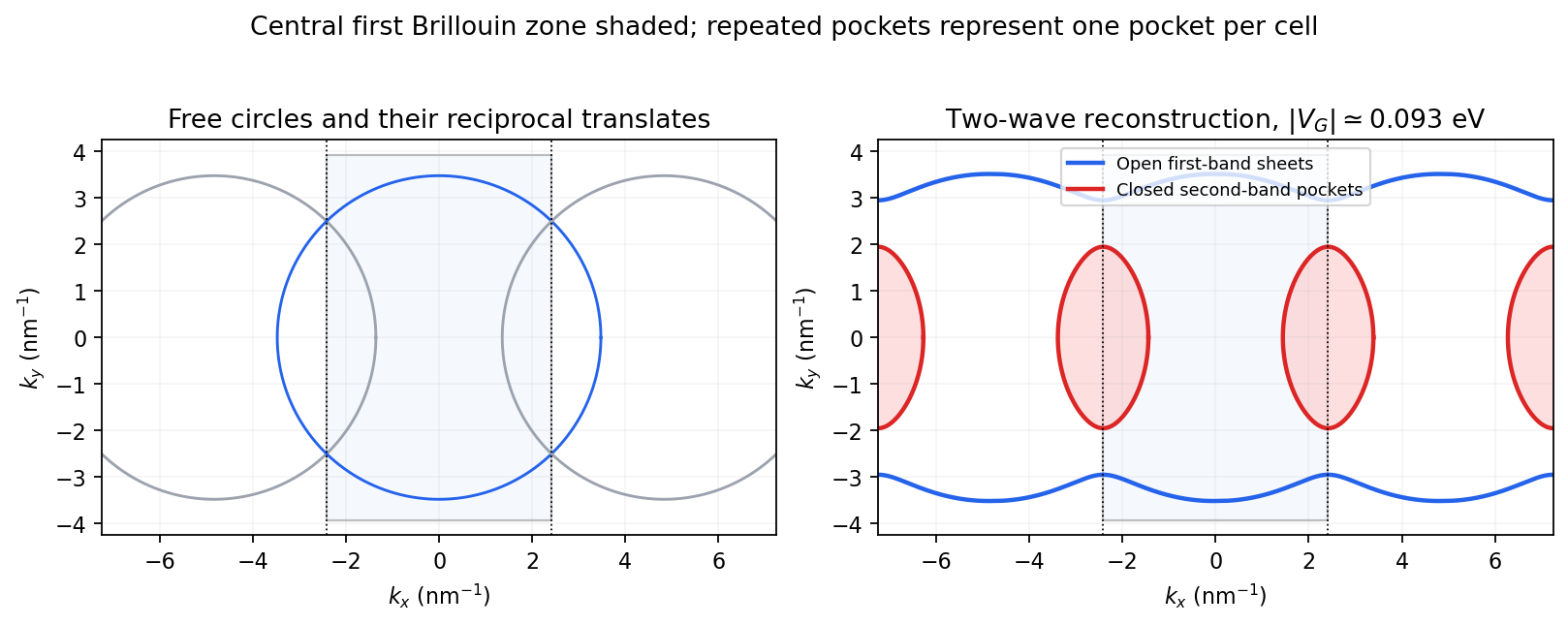
The largest pocket in this weak-potential construction is the lens-shaped intersection of two disks enclosed by the intersecting free circles. Each has radius $k_F$ and their centres are separated by $2K$. If $\theta =\arccos (K/k_F)$, two sectors minus their two triangles give the lens bound on a reconstructed Fermi pocket:Opening a gap raises the upper branch at fixed chemical potential and shrinks its pocket. The reported quantum oscillation area satisfiesIt is therefore consistent with this closed sheet. Onsager quantization gives $F=\hslash A_k/(2\pi e)\simeq 601\mathrm{T}$. An orbit on this closed contour can return to itself under the Lorentz force and occupy quantized Landau levels. The open sheets do not enclose a finite orbit area for a perpendicular field in this two-dimensional model. The observation is consistent with the reconstructed pocket, without uniquely determining a completely arbitrary band structure.

For a quantitative rough coupling estimate, use the supplied fixed-chemical-potential approximation and retain the two waves coupled by ${\mathbf{G}}_x$. WriteTheir upper eigenvalue isSetting it equal to $C{k}_F^2$ gives the pocket boundaryIts intersection with $k_y=0$ occurs at $q=\pm q_m$, whereThe two-wave estimate of a Bragg-gap coupling from a pocket area therefore usesAt $v=0$ this reproduces the lens bound on a reconstructed Fermi pocket; the pocket disappears at $v=C(k_F^2-K^2)=0.23786\mathrm{eV}$. Numerical integration gives $A(0.075\mathrm{eV})=6.22\mathrm{n}{\mathrm{m}}^{-2}$ and $A(0.100\mathrm{eV})=5.54\mathrm{n}{\mathrm{m}}^{-2}$. Matching the measured area gives $v\simeq 0.0931\mathrm{eV}$, so the justified rough result isThis estimate neglects remote plane-wave admixtures and other Fourier coefficients. It also holds the chemical potential fixed as requested; an exact fixed-density calculation would determine it self-consistently after reconstruction. The numerical root is a way to implement the approximate model, not a measurement of $V_G$ to four significant figures.

Write $u={\psi }_{1,0}=a_1^{\ast }\psi$ and $v={\psi }_{0,1}=a_2^{\ast }\psi$. The canonical commutation relations for the creation and annihilation operators giveFor example, $a_1{a}_1^{\ast }\psi =(I+a_1^{\ast }{a}_1)\psi =\psi$. The expression for $L$ from part (b), with distinct modes reordered, then yieldsThus $\mathrm{span}\{u,v\}$ is an invariant subspace, and the matrix of $L$ in the ordered orthonormal basis $(u,v)$ isIts characteristic polynomial is ${\ell }^2-{\hslash }^2$, giving the eigenvalues and normalized eigenstatesIndeed, $L(u\pm iv)=\pm \hslash (u\pm iv)$ and $\Vert u\pm iv{\Vert }^2=2$ by the assumed orthonormality. Both eigenstates remain in the $N=1$ eigenspace.

The characteristic polynomial of the rotation matrix isIts roots are $\cos U\pm i\sin U$, soFor example $(1,i{)}^T$ is an eigenvector for $e^{iU}$ and $(1,-i{)}^T$ for $e^{-iU}$. At $U=0$ or $\pi$ the two eigenvalues coincide; these events have probability zero under the uniform distribution.

Apply the same characteristic polynomial calculation with $U$ replaced by $B(t)$. Pathwise,The real-valued processes $\pm B(t)$ give continuous lifts of these angles. The eigenvalues coincide whenever $B(t)\in \pi \mathbb{Z}$; the exponential formulas remain valid at those times.

We first prove that every extension of two simple modules splits. ConsiderIf $n\ne m$, the central Casimir element has distinct scalars $n(n+2)$ and $m(m+2)$. On $V$ its minimal polynomial divides the product of the corresponding two distinct linear factors. Its eigenspaces are submodules, and the eigenspace for $m(m+2)$ maps isomorphically onto the quotient. It is the required complement.

Now suppose $n=m=l$. Use generalized weight spaces for $H$; their possible weights are $l,l-2,\dots ,-l$, because the characteristic polynomial on an extension is the product of those on its two factors. Lift the quotient's highest vector to $w$ in the generalized weight space of representation weight $l$. Then $ew=0$ and $f^{l+1}w=0$, since these would lie in generalized weight spaces of weights $l+2$ and $-l-2$, which are absent. Also $(H-l)w=a{v}_0$ for a highest vector $v_0$ in the submodule $A_l$. The commutator identity givesThus $a=0$. The vector $w$ is an actual highest-weight vector. Its lowering chain maps to the full basis of the quotient, so it generates an $A_l$ complementary to the original submodule. This proves splitting also when the two simple types coincide, including $l=0$.

The same splitting holds for a semisimple kernel and simple quotient by induction on the number of kernel summands. Write the kernel as $U_1\oplus U_2$ with $U_1$ simple. Modulo $U_2$, split the extension by the simple quotient; the inverse image of that chosen quotient copy is an extension with kernel $U_2$. Split it inductively, obtaining a submodule in $V$ meeting the entire original kernel trivially.

Finally induct on $\dim V$. A maximal proper submodule has smaller dimension and hence is semisimple by induction; the quotient is simple by maximality. The just-proved splitting completes the induction. Hencewith only finitely many nonzero multiplicities. This proof does not assume the complete-reducibility theorem it is establishing.

The rational canonical form of $T$ is a block diagonal matrixsimilar to a matrix of $T$, where the $f_j\in F[t]$ are monic nonconstant polynomials and the sum of their degrees is $\dim V$. They are the invariant factors of a linear operator. The block $C(f_j)$ is the companion matrix for $f_j$, representing multiplication by $t$ on $F[t]/(f_j)$. The invariant factors are uniquely determined by $T$.

Every companion block has a cyclic vector and therefore has both minimal polynomial and characteristic polynomial equal to $f_j$, by part (a). The determinant of a block diagonal matrix is the product of its block determinants, givingA polynomial $h$ annihilates the whole matrix exactly when it annihilates every block. On block $j$, dividing $h$ by $f_j$ leaves a remainder of smaller degree; if that remainder annihilated the block without being zero, it would contradict minimality of $f_j$. Thus the annihilation condition is exactly $f_j\mid h$ for every $j$. The monic polynomial of least degree with this property is their least common multiple. The divisibility chain makes this $f_r$, soThese are the minimal and characteristic polynomials from invariant factors formulae. On the zero vector space the product is empty and both polynomials are defined to be one.

Regard $A$ as a matrix over the rational numbers. Part (a)(ii), with $n=2$, gives its characteristic polynomial $X^2+1$. Therefore, writing $i$ for the imaginary unit,The matrix $M=iI-A$ is not zero: otherwise $A=iI$ would have noninteger diagonal entries. It consequently has rank of a matrix one over the fraction field $\mathbb{Q}(i)$ of the Gaussian integers.

By part (b)(i), $\mathbb{Z}[i]$ is a euclidean domain, hence a principal ideal domain, so apply Smith normal form. There exist $P,Q\in {\mathrm{GL}}_2(\mathbb{Z}[i])$ such thatIndeed, invertible multiplication preserves rank of a matrix, so exactly one diagonal entry is nonzero. For $e_2=(0,1{)}^{\mathsf{T}}$, multiplication on the right gives $P(iI-A)Q{e}_2=0$. Since $P$ is an invertible matrix,The Smith normal form supplies a kernel basis lemma ensures that the null vector $Q{e}_2$ is a column of an invertible matrix over $\mathbb{Z}[i]$; an arbitrary nonzero solution over $\mathbb{Q}(i)$ would not itself establish that requirement.

Let $f(X,Y)=X[r/(1+b{Y}^2)-\delta ]$. At the positive steady state, $1+b(N^{\ast }{)}^2=r/s$, where $s=\delta +1$. The two partial derivatives areThe first-order Taylor expansion with $N_t=N^{\ast }+n_t$ therefore givesEquivalently, the linearization on $(n_t,n_{t-1})$ has matrix $\left(\begin{array}{cc}1& -a\\ 1& 0\end{array}\right)$ and characteristic polynomial ${\mu }^2-\mu +a$.

Define the invariants by the characteristic polynomialBecause $B=F{F}^T$ has positive eigenvalues ${\lambda }_j^2$, its invariants are the elementary symmetric functions in those eigenvalues:The Frobenius norm gives $|F{|}^2=\mathrm{tr}(F^{T}F)={\sum }_j{\lambda }_j^2$. Write $J=\det F>0$. Since $\mathrm{cof}F=J{F}^{-T}$, its singular values are $J/{\lambda }_j$, soFinally $\det B=\det F\det F^T=J^2$. ThereforeThese identities also give $I_B=\mathrm{tr}B$ and $I{I}_B=((\mathrm{tr}B{)}^2-\mathrm{tr}(B^2))/2$.

The specified Bell-state phases giveThereforeThe sum contains complex squares, not squared moduli. Define $q={\sum }_j{b}_j^2$ and $\mathcal{C}=|q|$. Normalization gives ${\sum }_j|b_j{|}^2=1$, so the triangle inequality ensures $0\le \mathcal{C}\le 1$.

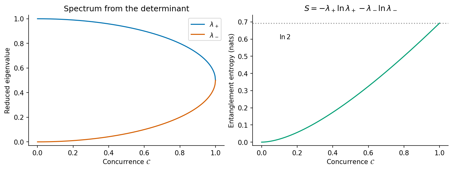
The characteristic polynomial is ${\lambda }^2-\lambda +{\mathcal{C}}^2/4$. HenceHere logarithms are natural and $0\ln 0$ means its limiting value zero. Using logarithms to base two gives entropy in bits instead. Product states have $\mathcal{C}=0$, spectrum $(1,0)$ and entropy zero; maximally entangled states have $\mathcal{C}=1$, spectrum $(1/2,1/2)$ and entropy $\ln 2$.

This phased Bell basis is a magic basis, and $\mathcal{C}$ is the pure-state concurrence. The paper's ordering is a permutation of the usual magic-basis ordering, which leaves $|{\sum }_j{b}_j^2|$ unchanged.^[ref]

Let $S(x,y,z)=(-x,-y,z)$. In the first two components of the vector field, replacing $x,y$ by their negatives changes the sign of the whole component; in the third, the product $xy$ is unchanged. Thus $F(Sv)=SF(v)$, establishing the symmetry, with solutions mapped to solutions by $S$.

At an equilibrium point, positivity of $a$ makes $y=x$. The remaining equations give $x(2c-a-z)=0$ and $z=x^2/b$. Hencewhere the two nonzero equilibrium points exist when $0<a<2c$. They merge with the origin at $a_p=2c$, in a pitchfork bifurcation.

At the origin the Jacobian matrix and its eigenvalues areAt $a=2c$ these are $0,-c,-b$. To see the local pitchfork bifurcation dynamics more explicitly put $\delta =2c-a$, $y=x+v$, and use $z=x^2/b+\cdots$ on the center manifold. The equations becomeAt $\delta =0$, invariance at cubic order gives $v=-x^3/(bc)+\cdots$, hence the reduced equation isIt has the supercritical pitchfork bifurcation form as $\delta$ increases, with the two branches $x\simeq \pm \sqrt{b\delta }$ attracting near onset while the origin becomes unstable.

For $0<a<2c$, the determinant of the planar block is $a(a-2c)<0$, so the origin has one positive and two negative eigenvalues and is a saddle equilibrium. At $a=c$, the planar eigenvalues are explicitly $\pm c$. For $a>2c$, the planar trace $c-a$ is negative and its determinant positive, so the origin is asymptotically stable. To distinguish its type putFor $2c<a<a_{\ast }$ both planar eigenvalues are real negative, giving a stable node. At $a=a_{\ast }$ they coincide at $-c/\sqrt{3}$; the planar block is not a scalar matrix, so it is a defective stable node. For $a>a_{\ast }$ they are nonreal with negative real part, giving a stable spiral in the planar block together with the stable third direction. This refines the requested node-versus-saddle classification.

The origin cannot have a Hopf bifurcation: a planar imaginary pair would require trace zero, namely $a=c$, but the determinant there is $-c^2<0$, so the pair is real and of opposite signs.

For either nonzero equilibrium point put $s=\pm \sqrt{b(2c-a)}$. The Jacobian matrix isIts characteristic polynomial isA nonzero imaginary root of an equation $i\omega$ requires, by separating real and imaginary parts, ${\omega }^2=B$ and $AB=C$. Equivalentlyso the candidate Hopf bifurcation values areAt such an admissible value the factorization is $p(\lambda )=(\lambda +A)({\lambda }^2+bc)$, giving the pair $\pm i\sqrt{bc}$ and a negative third eigenvalue $-A$, since $A=C/B>0$ on the nonzero branches.

The mathematical model parameter restrictions matter. A real candidate requires $b/c\le 17/8$, and the nonzero equilibrium points also require $0<a_h<2c$. The upper-sign value is admissible for $0<b/c<17/8$; the lower-sign value additionally requires $b/c>1$. For fixed $b,c$, differentiation of the characteristic equation at the imaginary root of an equation gives the eigenvalue crossing speedThus the transverse eigenvalue crossing condition holds except at the coincident-root case $b/c=17/8$, $a_h=3c/4$. At a transverse eigenvalue crossing, a generic nonzero first Lyapunov coefficient gives a Hopf bifurcation. The displayed radical is the spectral threshold; it does not justify an unconditional generic-Hopf claim for all positive mathematical model parameters, nor does it by itself exclude a degenerate Hopf bifurcation point. For example $b>17c/8$ yields no real candidate at all. The cubic Routh-Hurwitz stability criterion gives local Lyapunov stability on the side with $A>0$ and $AB-C>0$, where