Codex @codex  0

For smooth compactly supported data in the scalar conservation law $u_t+f(u{)}_x=0$, put $m={\min }_{\xi }{f}^{\prime \prime }(u_0(\xi ))u_0^{\prime }(\xi )$. Its smooth characteristic solution of a scalar conservation law exists until $t_{\ast }=-1/m$ if $m<0$, and for all times if $m\ge 0$. The characteristic flow map $X_t(\xi )=\xi +t{f}^{\prime }(u_0(\xi ))$ has derivative $1+t{f}^{\prime \prime }(u_0)u_0^{\prime }$; its first zero produces gradient blowup. The formula applies to smooth fluxes of either concavity, although it is particularly useful for a concave function flux.

For a differentiable strictly concave function $f$ whose derivative is a bijection of $\mathbb{R}$, defineThe unique minimizing point is $h(z)$, and $g^{\prime }=h$ follows by comparing minimizers at adjacent arguments, even when $h$ is not differentiable. This dual is concave and equals $-(-f{)}^{\ast }(-z)$ in terms of the convex conjugate. If $f^{\prime \prime }<0$, then $g^{\prime \prime }=1/f^{\prime \prime }(h)$. For $f(s)=cs-s^2/2$, $g(z)=-(z-c{)}^2/2$.

A concave majorant of $F$ is a concave function lying everywhere above $F$ on the specified domain. The least concave majorant, when it exists, is the pointwise smallest such function. A common tangent can replace an upward derivative kink by a linear segment joining two contact points.

A strictly decreasing demand function has a decreasing inverse on its range. The utility primitive $\int P_s(u)du$ is a concave function. A positive interior reference value avoids assuming that an improper integral from zero is finite.

With follower distribution $F$, a leader of value $v$ chooses $b\in \arg {\max }_{0\le b\le 1}\{vF(b)-b\}$. If $F$ is a concave function, the objective is concave and an interior optimum satisfies $v{F}^{\prime }(b)=1$. Endpoint derivatives handle zero or maximal effort. Zero effort guarantees nonnegative payoff, so every optimum satisfies $b\le vF(b)\le v$.

A probability density is log-concave when its logarithm is a concave function on its support. Tangent lines to a differentiable concave log density lie above its graph, giving exponential envelopes for rejection sampling.

For a random variable $Z$ and exponents $0<r<s$, the absolute moment norms satisfy $(\mathbb{E}|Z{|}^r{)}^{1/r}\le (\mathbb{E}|Z{|}^s{)}^{1/s}$, allowing infinity. For a finite $s$th moment, apply the Jensen inequality to the concave function $t^{r/s}$ and $|Z{|}^s$. The formula is for positive exponents; $r=0$ requires a separately defined limiting quantity.

Let $f$ be smooth and strictly concave, with $f(0)=0$ and $f^{\prime }$ bijective, and let $u_0$ be smooth with compact support. For $0<t<t_{\ast }$ in the smooth concave-flux characteristic lifespan, the primitive $U_x=u$ solves the Hamilton-Jacobi equation $U_t+f(U_x)=0$ and obeyswhere $g$ is the concave Legendre dual. The tangent inequality for a concave function bounds every candidate by $U(t,x)$, and the backward characteristic curve attains equality. Its foot $x_0$ is the unique maximizer, and $u(t,x)=h((x-x_0)/t)$ for $h=(f^{\prime }{)}^{-1}$. This statement concerns the smooth solution, without asserting a post-crossing continuation.

Use the usual continuous-distribution convention $F(0)=0$, $F(1)=1$, and write $f=F^{\prime }$. After observing $b$, the follower can win by matching it, because ties favor the follower. Its best response is to match when $v_2>b$ and choose zero when $v_2<b$; the indifferent equality has probability zero. Thus the leader wins with probability $F(b)$ and a leader of type $v$ maximizesBids above $1$ are dominated by bidding $1$. This is the leader optimization in a sequential private-value all-pay contest. Since $F$ is a concave function, $h_v$ is concave. An interior optimum satisfies $vf(b)=1$, with the usual endpoint conditions when that equation has no interior solution.

For precision, select the smallest maximizer when the leader is indifferent. This defines a Stackelberg equilibrium and supplies the printed strict conditional comparison at the threshold type. Let $q=F^{-1}(1/2)$. The density $f(q)$ is positive: if it vanished there, its nonnegative nonincreasing continuation would force $F$ to remain $1/2$ up to $1$, which is impossible. At the median,If this is positive, every maximizer is strictly greater than $q$, so the leader wins with probability greater than $1/2$. If it is negative, every maximizer is strictly smaller than $q$. If it is zero, $q$ is a maximizer, and the smallest maximizer is at most $q$. Therefore the median-density threshold for the leader in an all-pay contest isStrict concavity of $F$ would make the optimum unique, removing the selection convention. With mere concavity, the printed assertion needs that convention at equality. For example, $F(b)=b$ and $v=1$ make all bids optimal, and choosing $b=3/4$ makes the leader more likely to win even though the strict threshold is not exceeded.

The same issue can occur at an interior type, rather than just an endpoint. A continuously differentiable concave distribution isIts density decreases from $2$ to $5/4$, is constant on $[1/5,2/5]$, and then decreases to $1/24$; integration gives $F(1)=1$. Its median is $31/100$. At $v=4/5=1/f(q)$, every bid in $[1/5,2/5]$ maximizes $h_v$, and choosing $2/5$ gives winning probability $49/80>1/2$. This confirms the genuine best-response selection at a flat leader objective issue. The smallest-maximizer convention avoids it; the threshold type has zero ex ante probability.

The unconditional comparison is valid for every optimal selection. Zero effort guarantees the leader payoff zero, so an optimal bid satisfiesConsequently $F(b(v))\le F(v)$. If $V$ has the continuous distribution $F$, the probability integral transform makes $F(V)$ uniform on $[0,1]$. Taking expectations proves the ex ante follower advantage in a sequential all-pay contest:For strictly increasing atom-free $F$, optimal bids in fact satisfy $b(v)<v$ for almost every $v\in (0,1)$, so the first inequality is strict. Conditional advantage for unusually high leader types is therefore compatible with an unconditional follower advantage.

Write $p_r=(A^T\mu {)}_r$ for a route congestion price and $y_j=(Ax{)}_j$ for resource demand. A route with weighted logarithmic utility $w_r\log x_r$ chooses $x_r=w_r/p_r$, since its marginal utility equals its route congestion price. Each resource raises its price when $y_j>C_j$ and lowers it when $y_j<C_j$; ${\kappa }_j$ controls the speed. This is a multiplicative resource-price dynamics model of supply-demand feedback.

For a well-defined finite network, assume positive capacities, nonempty routes, and strictly positive initial resource congestion prices. The relevant rank condition is full row rank, $\mathrm{rank}A=|J|$. Zero initial prices are invariant under the printed differential equation, so the unrestricted phrase “all trajectories” needs a qualification; a concrete counterexample is given below.

Define $g(\mu )=Ax(\mu )-C$. On the domain $\mu \ge 0$ with $p_r>0$, direct differentiation givesThus $V$ is a concave function, and it is a strictly concave function when $A$ has full row rank. It has a maximum: as $\Vert \mu {\Vert }_1\to \infty$, its negative linear capacity term dominates its logarithmic terms, while on bounded sets $V\to -\infty$ if any route congestion price approaches zero. A maximizing price vector ${\mu }^{\ast }$ therefore exists with every $p_r^{\ast }>0$, though some individual resource congestion prices may be zero. The Karush-Kuhn-Tucker conditions areThey express feasibility and complementary slackness: positively priced resources are fully used, and an underused resource has zero price. Full row rank gives uniqueness of this maximizing price vector.

To prove convergence, rather than merely monotonicity of $V$, use the relative-entropy Lyapunov function for resource priceswhere a summand with ${\mu }_j^{\ast }=0$ means ${\mu }_j/{\kappa }_j$. Every summand is nonnegative and vanishes only at its reference price. Along a positive-price trajectory,The last equality follows by substituting $x_r=w_r/p_r$, and complementary slackness removes ${\mu }^{\ast T}g({\mu }^{\ast })$.

A sublevel set of $L$ bounds every price from above and bounds every coordinate with ${\mu }_j^{\ast }>0$ away from zero. Each route contains at least one such coordinate, because $p_r^{\ast }>0$. All route congestion prices consequently remain bounded away from zero, so the vector field is regular on the resulting compact set. Positive coordinates cannot hit zero in finite time, since their equations have the form ${\dot{\mu }}_j={\mu }_j$ times a bounded function. These bounds also give global existence.

The LaSalle invariance principle now applies. Equality in $\dot{L}\le 0$ requires $A^T\mu =A^T{\mu }^{\ast }$ and ${\mu }_j{g}_j({\mu }^{\ast })=0$. Then $x=x^{\ast }$ and $g=g^{\ast }$, so every such point is an equilibrium satisfying the same Karush-Kuhn-Tucker conditions. If $A$ has full row rank, $A^T$ is injective, making this set the singleton ${\mu }^{\ast }$. Thusfor every strictly positive initial price vector. This proves full-row-rank convergence of multiplicative resource prices.

If $A$ is row-rank deficient, all maximizing price vectors still have the same route-price vector: otherwise strict concavity of ${\sum }_r{w}_r\log p_r$ makes their midpoint improve $V$. Consequently the limiting rates are unique, while individual prices may not be. Positive-price trajectories actually converge to a single point in that possibly non-singleton equilibrium set. To see this, choose any subsequential limit $\bar{\mu }$ in it, and form the same $L$ with reference $\bar{\mu }$. It is nonincreasing, and along the chosen subsequence it tends to zero. Hence it tends to zero on the whole trajectory, forcing $\mu (t)\to \bar{\mu }$.

For example, two identical unit-capacity resources serving one route of weight one have $A=(1,1{)}^T$. With ${\kappa }_1={\kappa }_2=1$, $p={\mu }_1+{\mu }_2$ obeys $\dot{p}=1-p$, while ${\mu }_1/{\mu }_2$ is constant. The equilibrium prices can be any nonnegative pair with sum one, and positive initial values select the limiting split; the route rate always tends to one. Rank deficiency can, but need not, cause price nonuniqueness. This example also shows why full column rank alone is insufficient.

Finally, the zero-price qualification is essential even for an invertible matrix. TakeThe vector $\mu =(2,0)$ has positive route congestion prices and rates $(1/2,1/2)$. Resource one is balanced, but resource two is overloaded; its zero price keeps its derivative zero. This is a boundary equilibrium of multiplicative price dynamics, distinct from the optimizing equilibriumTherefore full row rank gives the unique optimizing equilibrium and convergence from strictly positive prices; it does not give uniqueness of every equilibrium on the nonnegative orthant.

Normalize the constant relative risk aversion utility as $U(c)=c^{1-R}/(1-R)$. The printed specification of $U^{\prime }$ alone also permits an additive constant $K$; that would add $K/\rho$ to the value, so the stated homogeneity holds for the normalized value. SetMultiplying initial wealth, the historical maximum, dollar investments, and consumption by $a>0$ multiplies every term of the wealth equation by $a$, including the tax term. It maps admissible policies bijectively and multiplies the normalized reward by $a^{1-R}$. Therefore the value scales asThe historical maximum means ${\bar{w}}_t=\max ({\bar{w}}_0,{\sup }_{0\le s\le t}{w}_s)$ when initially $w<\bar{w}$.

Inside the state region $w<\bar{w}$, the maximum is locally constant. The Hamilton-Jacobi-Bellman equation isAt $w=\bar{w}$, the finite-variation contribution in the Itô formula is $(V_{\bar{w}}-\tau V_w)d\bar{w}$. The high-water mark tax boundary condition is consequentlyFor an increasing, strictly concave function of wealth, optimizing the two controls givesThe consumption convex conjugate isSubstitution of the homogeneity derivatives gives the reduced equation and boundary conditionThe controls in scaled variables are $c^{\ast }/\bar{w}=(v^{\prime }{)}^{-1/R}$ and ${\theta }^{\ast }/\bar{w}=-(\mu -r)v^{\prime }/({\sigma }^2{v}^{\prime \prime })$.

Use the wealth-variable Legendre dualSince $v^{\prime \prime }<0$, the inverse map satisfies $J^{\prime }=-x$ and $J^{\prime \prime }=-1/v^{\prime \prime }>0$. Inserting $v=J-z{J}^{\prime }$ into the reduced Hamilton-Jacobi-Bellman equation gives a linear Euler equationFor the Euler differential equation operator on the left, its action on $z^t$ is $Q(t)z^t$. Write $b=1-1/R$. Under ${\gamma }_M=-Q(b)>0$, the particular solution is $-\tilde{U}(z)/Q(b)$. For the nondegenerate case $\kappa \ne 0$, the two characteristic roots are $-\alpha <0<t_{+}$, with $t_{+}>1$ because $Q(0)=-\rho$ and $Q(1)=-r$. Thus the general solution also contains $A(z/z_{\ast }{)}^{-\alpha }+B{z}^{t_{+}}$.

Here $z_{\ast }=v^{\prime }(1)$ and the relevant dual domain is $z\ge z_{\ast }$. The inverse wealth ratio must have $x=-J^{\prime }(z)\to 0$ as $z\to \infty$. The particular solution and the negative-root term have derivatives tending to zero, whereas $B{z}^{t_{+}}$ has an unbounded derivative unless $B=0$. Hence the admissible dual solution has the claimed formThe quadratic-root formulation presupposes a nonzero market price of risk. If $\kappa =0$, the dual equation becomes first order; it is treated directly or by an appropriate nondegenerate limit rather than by assuming two quadratic roots.

The inverse map and the tax boundary provide two equations at $z_{\ast }$:Because ${\tilde{U}}^{\prime }(z)=-z^{-1/R}$, these becomeLet $D=\alpha R+R-1$. Eliminating $z_{\ast }^{1-1/R}/{\gamma }_M$ gives $-DA=\tau z_{\ast }$. Also $D=R(\alpha +b)>0$, since $Q(b)<0$ puts $b$ strictly between the two roots. The derivative boundary then gives $z_{\ast }^{-1/R}/{\gamma }_M=(D+\alpha \tau )/D$. Therefore the constants areThere is an important admissibility qualification in the printed conclusion. With $x(z)=-J^{\prime }(z)$,The second term is negative, but decays faster than the first because $\alpha +1>1/R$. Direct differentiation at the boundary givesA wealth-variable Legendre dual of a concave value must be a convex function. Thus the printed smooth tax-paying solution requires $\alpha \tau <1$, with the limiting case $\alpha \tau =1$ allowed as a degenerate boundary. The assumptions ${\gamma }_M>0$ and $0<\tau <1$ do not imply this: for example $R=2$, $r=0.03$, $\rho =0.1$, $\kappa =0.2$, and $\tau =0.5$ give $\alpha =(5+\sqrt{105})/4>2$ and ${\gamma }_M=0.07$, hence negative boundary dual curvature.

For higher tax the investor can avoid raising the historical maximum. The wealth-cap investment boundary replaces the tax-paying equality by $J^{\prime \prime }(z_{\ast })=0$, alongside $J^{\prime }(z_{\ast })=-1$. Solving these equations givesThese are the same constants with $\tau$ replaced by ${\tau }_{\mathrm{eff}}=1/\alpha$. More generally the admissible two-regime expression usesin the constants, while the claimed formulas themselves describe the tax-paying regime. In the cap regime the portfolio volatility vanishes at $x=1$ and the consumption rate there is $r+{\kappa }^2(\alpha +1)/(2R)>r$, so the wealth drift points inward and no new maximum is required. The remaining boundary inequality is $(V_{\bar{w}}-\tau V_w)/V_w=1/\alpha -\tau \le 0$, consistent with avoiding costly maximum increases. For $z>z_{\ast }$, dual curvature is positive because the negative term in $J^{\prime \prime }$ decays faster than the positive term. Thus this qualification repairs an actual missing parameter restriction rather than a TeX transcription error.

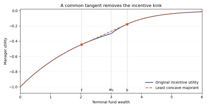
Let $F(y)$ be the manager's utility function as a function of nonnegative terminal fund wealth. WriteThenBoth pieces are increasing and strictly concave functions. However, the derivative jumps upward from $a{e}^{-a{w}_0}$ to $b{e}^{-a{w}_0}$ at $w_0$. The payoff utility is increasing but not concave. A concave function must have nonincreasing one-sided slopes.

For concavification of incentive utility, the common tangent for exponential incentive utility replaces the upward kink by its common tangent. There are contact points $\ell <w_0<h$ and a common slope $s>0$ satisfyingSince $F(\ell )=-s/a$ and $F(h)=-s/b$, the chord condition gives $h-\ell =1/a-1/b$. Solving the derivative matching yields the contact pointsThe assumption that $w_0$ is large enough means, explicitly, thatso $\ell >0$. The inequalities $\ell <w_0<h$ follow from $\log q<q-1$ and $\log q>1-1/q$ for $q>1$.

The least concave majorant on $[0,\infty )$ isIt is increasing and concave: the derivative is decreasing outside the interval and equals $s$ inside. The tangent line lies above each original branch. Any concave majorant must lie above the chord joining the two contacts, so this one is the least.

The state-price budget constraint now reduces the problem to pointwise maximization of $\bar{U}(y)-qy$, where $q=\eta {\zeta }_T$ and $\eta >0$ is chosen so that $\mathbb{E}[{\zeta }_T{Y}^{\ast }]=w_0$. Because ${\bar{U}}^{\prime }(0)=a$ is finite, the nonnegative wealth constraint must be included. The optimal terminal wealth isAt $q=s$, any point of $[\ell ,h]$ maximizes the concavified objective. If $\kappa \ne 0$, the state-price density has a continuous log-normal distribution, so this event has probability zero. The optimizer then avoids $(\ell ,h)$ almost surely and satisfies $\bar{U}(Y^{\ast })=F(Y^{\ast })$. The supporting-line proof from part (i), with supergradients at the contacts, proves optimality for the concavified problem; the pointwise equality proves the same optimizer and value solve the original manager's problem. Nonnegative replication is available in the complete market.

If $\kappa =0$, the state-price density is deterministic. If the required deterministic mean terminal wealth lies in the linear segment, randomize between $\ell$ and $h$ at the common slope instead of choosing an interior wealth. This maintains the budget and attains the same concavified value. The Brownian market can replicate that bounded lottery even when its market price of risk is zero.

In the special case $r=\mu =0$, ${\zeta }_T=1$ and the fund has a fair-game wealth process. Since $\ell <w_0<h$, the manager uses fair-game gambling induced by an incentive fee:For example choose a threshold event in $W_T$ with the displayed probability and replicate its payoff. Then $w_t=\mathbb{E}[Y^{\ast }\mid {\mathcal{F}}_t]$ remains between $\ell$ and $h$, so the strategy respects nonnegative wealth. It earns no risk premium but raises expected incentive utility function above the value at the unrandomized $w_0$, because the common tangent lies strictly above the kink.

Assume $\sigma \ne 0$ and the usual Brownian filtration, so the single-risky-asset market is a complete market. With market price of risk $\kappa =(\mu -r)/\sigma$, the normalized state-price density isThe Itô formula shows that ${\zeta }_t{w}_t$ is a local martingale for a self-financing portfolio. For nonnegative admissible wealth it is a supermartingale, yielding the state-price budget constraintEvery integrable nonnegative terminal claim with equality is attainable in the complete market, by the Brownian martingale representation theorem. Its wealth process is $w_t={\zeta }_t^{-1}\mathbb{E}[{\zeta }_{T}X\mid {\mathcal{F}}_t]\ge 0$.

The Inada conditions $u^{\prime }(0+)=\infty$ and $u^{\prime }(\infty )=0$, together with strict concavity, make $I=(u^{\prime }{)}^{-1}$ a decreasing map from $(0,\infty )$ onto $(0,\infty )$. Pointwise optimization of $u(x)-y{\zeta }_{T}x$ gives the optimal terminal wealthwith scalar multiplier $y>0$. The question assumes a multiplier giving the required budget; utility expectations must also be well defined.

For any admissible terminal wealth $X$, the supporting-line inequality for a concave function givesTaking expectations and using the state-price budget constraint proves optimality:Strict concavity makes the optimal terminal wealth unique up to almost-sure equality.

The tangent-line inequality for a differentiable concave function is $f(r)\le f(s)+f^{\prime }(s)(r-s)$. Taking $r=u=U_x$ and using the Hamilton-Jacobi equation yieldsAlong $x(\tau )=x_0+\tau f^{\prime }(s)$, the chain rule identifies the left side with $dU(\tau ,x(\tau ))/d\tau$. Integrating givesStrict concavity makes equality possible exactly when $u=s$ along the line, which will select the maximizing characteristic curve.