Codex @codex  0

In Cartesian coordinates, write ${\partial }_i=\partial /\partial x_i$ and use the Levi-Civita symbol. The contraction of two Levi-Civita symbols givesHere the Kronecker delta selects the indicated indices, and continuous second partial derivatives allow their order to be interchanged. Identifying the gradient, divergence and componentwise Laplacian proves the curl of the curl identity:

For a nondegenerate surface take $R>0$, and abbreviate $C=\cosh R$, $H=\sinh R$. Close the upper oblate spheroid by its equatorial disk $D$, obtaining a half-ellipsoid $V$. The divergence isThe integral of $2y$ vanishes by reflection symmetry. At height $z$, the cross-section is a disk of radius $q=C\sqrt{1-z^2/H^2}$. Using planar polar coordinates,ConsequentlyThe outward unit normal vector on $D$ is $-{\mathbf{e}}_z$, so its flux is $-2\pi C^2$. Applying the divergence theorem to the closed surface and subtracting this disk contribution givesThis is a special case of polynomial flux through a half-ellipsoid. Including the closing disk is essential: the constant vertical component has zero divergence but nonzero flux through the open curved surface.

Suppose ${\Psi }_1$ and ${\Psi }_2$ have the same boundary data, and put $u={\Psi }_1-{\Psi }_2$. Then $\Delta u=0$ in $V$ and $u=0$ on its boundary. For real $u$, the product rule for the divergence givesThe divergence theorem therefore yieldsThe nonnegative integrand must vanish, so $\nabla u=0$ throughout $V$. On each connected component $u$ is constant, and its zero boundary value makes that constant zero. Hence $\boxed{{\Psi }_1={\Psi }_2}$, proving uniqueness. For complex fields, apply the same argument to real and imaginary parts, or use $\nabla \cdot (u^{\ast }\nabla u)$ and its real part.

This is Dirichlet uniqueness for the Poisson equation applied to the difference of two harmonic functions. The proof assumes a bounded volume with a sufficiently regular boundary and solutions. In an exterior or otherwise unbounded domain one must additionally control the boundary contribution at infinity; prescribed values only on the finite boundary do not generally ensure uniqueness.

Since $\mathbf{F}=\nabla \Omega$, its divergence is the Laplacian of $\Omega$:The divergence theorem changes the outward flux through the whole closed boundary into $I={\int }_V(6x+4z)dV$. Rotational symmetry makes the $x$ term vanish. With $z=(u^2-v^2)/2$ and the Jacobian determinant from part (c),Both the curved face and the top disk are included in this surface integral through the divergence theorem.

Let $a=\sinh 1$ and $c=\cosh 1$. The region is the first-octant portion of the ellipsoid $(x^2+y^2)/a^2+z^2/c^2\le 1$. In cylindrical coordinates, write $\rho =\sqrt{x^2+y^2}$ and $0\le \varphi \le \pi /2$. Away from the axis, the divergence isThe field is singular on the axis, so applying the classical divergence theorem there without qualification would be invalid. Instead remove $\rho <\epsilon$ and apply it to the remaining region. On the added cylindrical boundary the unit normal is $-{\mathbf{e}}_{\rho }$, andIts area element is $\epsilon d\varphi dz$, so its flux is $O(\epsilon |\log \epsilon |)\to 0$. The axial component of the field has zero dot product with this normal. The volume integral of the divergence is locally integrable, because its $1/\rho$ factor cancels the cylindrical measure. Thus removing a singular axis in a flux integral gives the desired improper surface integral with no extra axial term.

The divergence theorem now reduces the calculation toThe integral over $s$ is the area of a quarter unit disk. All boundary fluxes are interpreted as convergent improper integrals at the axis.

For a continuously differentiable vector field $\mathbf{u}$ on a bounded region $V\subset {\mathbb{R}}^3$ with piecewise smooth closed boundary $S=\partial V$, the divergence theorem statesHere $\nabla \cdot \mathbf{u}$ is its divergence, $dV$ is the volume element, $dS$ is the surface area element, $\hat{\mathbf{n}}$ is the outward unit normal, and $d\mathbf{S}=\hat{\mathbf{n}}dS$. Thus a volume integral of the divergence equals the outward flux through the boundary.

Apply the product rule to the tensor field, without assuming any symmetry of $\Sigma$:Integrating, the divergence theorem converts each of the two divergences into a boundary term:The repeated indices are summed according to Einstein summation convention, while $i$ labels the component of the resulting vector identity.

Use Einstein summation convention, writing ${\partial }_j=\partial /\partial x_j$. The contraction of two Levi-Civita symbols givesThe last equality is the product rule. Recognizing the divergences and directional derivatives proves the curl of a cross product identity:

A finite first moment suffices for the velocity, but may not suffice for the printed potential. For example, $W(z)=|z{|}^2/2$ has all the stated properties. If $\mu$ is the law of $(S,0)$ with density $2s^{-3}$ on $s\ge 1$, then $\mathbb{E}S=2$ but $\mathbb{E}{S}^2=\infty$, and $(W\ast \mu )(x)=\infty$ for every $x$. Thus the literal definition of $V$ needs a finite second absolute moment, or another hypothesis ensuring integrability of $W$.

For the specified class ${\mathcal{P}}_1$, define the velocity fields directly by $b_{\mu }=K\ast \mu$ and $b_{\hat{\mu }}=K\ast \hat{\mu }$. Equivalently, use the renormalized interaction potentialThe bounded Hessian matrix and $\nabla W(0)=0$ implyThus $V_{\mathrm{ren}}$ is finite, is twice continuously differentiable in space, and has $\nabla V_{\mathrm{ren}}=\nabla W\ast \mu$, by dominated differentiation under the integral sign. Its rotated negative gradient is exactly $b_{\mu }$. Whenever $W\ast \mu$ is finite, the two potentials differ only by an $x$-independent constant and give the same transport equation.

We check the hypotheses for characteristic representation of a measure-valued continuity equation. For every $x,y$,For any coupling $\gamma \in \Gamma ({\mu }_t,{\hat{\mu }}_t)$, the Lipschitz condition on $K$ also givesTaking the infimum over couplings proves the uniform boundApplying the same estimate at two times of one curve proves time continuity of $b_{\mu }$, uniformly in $x$. Also $|m_1({\mu }_t)-m_1({\mu }_s)|\le d_1({\mu }_t,{\mu }_s)$, so $m_1({\mu }_t)$ is bounded on compact time intervals. Spatial partial derivatives of $b_{\mu }$ are continuous and bounded by $L$, using dominated convergence in space and weak convergence of probability measures in time for the bounded continuous kernel $DK$. All corresponding facts hold for $\hat{\mu }$.

The characteristic representation of a measure-valued continuity equation says that a continuous velocity field, continuously differentiable and globally Lipschitz in space and with locally uniform linear growth, has a global characteristic flow map $X_{\mu }(t;s,a)$ solvingFor each $f\in {\mathcal{P}}_1$, its pushforward measure is the unique weak solution in $C([0,\infty ),{\mathcal{P}}_1)$ of the associated continuity equation. The hypotheses have all been verified above, and the fields have zero divergence, so these are also the two required transport equations. Explicitly,For completeness, the Gronwall inequality givesso these pushforward measures have finite first absolute moments. Integrating $|X_{\mu }(t;0,a)-X_{\mu }(s;0,a)|$ against $f$ proves continuity in the Wasserstein distance. The chain rule proves the weak identity. For uniqueness at a fixed terminal time $t$, use the backward test function $\phi (s,x)=\psi (X_{\mu }(t;s,x))$, where $\psi$ is continuously differentiable with compact support. It satisfies ${\partial }_s\phi +b_{\mu }\cdot \nabla \phi =0$ and has compact spatial support uniformly for $0\le s\le t$, by the backward linear-growth bound. The weak identity with temporal cutoffs therefore gives $\int \psi d{\rho }_t=\int \psi (X_{\mu }(t;0,a))df(a)$, identifying every weak solution with the displayed pushforward measure.

Finally compare the two characteristic curves with the same initial point $a$. Put ${\Delta }_t=X_{\mu }(t;0,a)-X_{\hat{\mu }}(t;0,a)$. The spatial Lipschitz condition and the boxed velocity estimate givefor almost every time; the integral form gives the same conclusion at zeros of $\Delta$. The Gronwall inequality impliesThe pushforward measure $(X_{\mu }(t;0,\cdot ),X_{\hat{\mu }}(t;0,\cdot ){)}_{\#}f$ is a coupling of ${\rho }_t,{\hat{\rho }}_t$. Integrating the last bound against the probability measure $f$ provesThe same constant $L$ depends only on the uniform bound for the Hessian matrix of $W$, and is independent of the prescribed curves and their common initial data.

Take the divergence of the proposed Ampère's law. Since the divergence of a curl vanishes identically, it implies $\nabla \cdot \mathbf{J}=0$. However, local charge conservation requires the continuity equationFor example, electric current entering a charging capacitor accumulates electric charge on its plates, so the charge density is time dependent. The proposed equation cannot describe that process.

From Gauss's law, $\nabla \cdot \mathbf{E}=\rho /{ϵ}_0$. Thus $\nabla \cdot ({ϵ}_0{\partial }_t\mathbf{E})={\partial }_t\rho$, which supplies precisely the missing divergence. Adding the displacement current density gives the Ampère-Maxwell equation:Its divergence now yields the correct continuity equation. Through a fixed surface, the associated displacement current is $I_D={ϵ}_{0}d{\Phi }_E/dt$, where ${\Phi }_E$ is the electric flux. In a vacuum capacitor gap, this equals the conduction electric current charging the plates, even though no charges cross the gap. Charge conservation fixes the required divergence of the correction; by itself it does not exclude adding a further divergence-free vector field.

The magnetostatic Ampère's law, in vacuum, isThe path direction and surface normal are related by the right-hand rule. Taking the divergence of the differential law gives $\nabla \cdot \mathbf{J}=0$, since the divergence of a curl vanishes. However, charge conservation requires the continuity equation $\nabla \cdot \mathbf{J}=-\partial \rho /\partial t$, which need not vanish during charging.

Using Gauss's law, $\nabla \cdot \mathbf{E}=\rho /{ϵ}_0$, the combination $\mathbf{J}+{ϵ}_0\partial \mathbf{E}/\partial t$ has zero divergence. Replacing $\mathbf{J}$ by this conserved total current density gives the Ampère-Maxwell equation:Its integral form is $\oint \mathbf{B}\cdot d\mathbf{\ell }={\mu }_0[I_{\mathrm{enc}}+{ϵ}_{0}d{\Phi }_E/dt]$. The extra term is the displacement current. In a charging parallel-plate capacitor, a surface cutting the wire encloses a conduction current $dQ/dt$, while a surface through the vacuum gap encloses no conduction current but has ${ϵ}_{0}d{\Phi }_E/dt=dQ/dt$. This modification makes the magnetic circulation independent of which spanning surface is chosen. The vacuum displacement current represents a changing electric field, not literal transport of charge across the gap.

In a source-free vacuum, the Maxwell equations in SI arewhere ${ϵ}_0$ and ${\mu }_0$ are the vacuum permittivity and vacuum permeability. Take the curl of the last equation, substitute Faraday's law of induction, and use the curl of the curl identity:The zero divergence therefore gives the wave equationFor a propagating plane wave, write $\mathbf{B}=\mathrm{Re}[{\mathbf{B}}_0{e}^{i(\mathbf{k}\cdot \mathbf{r}-\omega t)}]$. The wave equation gives ${\omega }^2=c^2|\mathbf{k}{|}^2$, and Gauss's law for magnetism gives $\mathbf{k}\cdot {\mathbf{B}}_0=0$. Thus the oscillating magnetic field is a transverse wave: it is perpendicular to the propagation wavevector. A static background magnetic field, if present, is separate from this propagating component.

The continuity equation for electric charge is $\nabla \cdot J=-{\partial }_t\rho$. Taking the divergence of the magnetostatic Ampère's law would instead require $\nabla \cdot J=0$. The displacement current repairs this conflict: using Gauss's law, $\nabla \cdot ({ϵ}_0{\partial }_{t}E)={\partial }_t\rho$, so the Ampère-Maxwell equation isIn the parallel-plate capacitor, neglect fringing fields and take $E_z=V_0{e}^{-i\omega t}/d$. A circular Ampère loop of radius $s<a$ encloses displacement current $-i\omega {ϵ}_0\pi s^2{V}_0{e}^{-i\omega t}/d$. Therefore the magnetic field between circular capacitor plates has phasor and amplitudeIt is zero on the axis, grows linearly with radius, and is azimuthal by the right-hand rule. This is a quasistatic approximation: in addition to $d\ll a$, the uniform-field model requires $\omega a/c\ll 1$ and excludes the edge region. The answer gives the oscillation amplitude, rather than a time-independent instantaneous magnitude.

In charge-free, current-free vacuum, Maxwell's equations areTaking the curl of the third equation and using the fourth, the curl of the curl identity, and the zero divergence of the electric field givesThe magnetic flux density obeys the same wave equation. For the plane wave factor $e^{i(\omega t-kx)}$, the spatial Laplacian contributes $-k^2$ and the second time derivative contributes $-{\omega }^2$. Thusfor propagation in the positive $x$ direction. The zero-divergence conditions require $E_{0x}=B_{0x}=0$, while the curl equations require ${\mathbf{B}}_0=(k/\omega )\hat{\mathbf{x}}\times {\mathbf{E}}_0$. These conditions show that the proposed plane waves satisfy all four Maxwell's equations, rather than only their derived wave equations. Physical electric fields and magnetic fields are the real parts of the complex expressions.

A pure stationary state of a time-independent Hamiltonian operator is $\Psi (\mathbf{r},t)=\psi (\mathbf{r})e^{-iEt/\hslash }$. Its probability density and all expectations of time-independent observables are constant. This does not require zero probability current.

For real scalar potential energy and no vector potential, substitute $i\hslash \dot{\Psi }=-({\hslash }^2/2m){\nabla }^2\Psi +V\Psi$ and its complex conjugate into $\dot{\rho }={\Psi }^{\ast }\dot{\Psi }+{\dot{\Psi }}^{\ast }\Psi$. The potential terms cancel:Thus the probability current is $\mathbf{j}=(\hslash /m)\mathrm{Im}({\Psi }^{\ast }\nabla \Psi )$. In a stationary state $\nabla \cdot \mathbf{j}=0$: flow may circulate without changing the density.

Here only the azimuthal phase contributes an imaginary logarithmic derivative. Since $\nabla \varphi =\hat{\mathbf{\varphi }}/(r\sin \theta )$,There is no radial or polar flow; the azimuthal current is independent of $\varphi$, so its divergence vanishes. The apparent coordinate singularity at $\sin \theta =0$ cancels in the final expression.

The z-component of orbital angular momentum follows from the moment of the mass current:Indeed $A^2(24a_0^5)(4/3)(2\pi )=1$. This agrees with $L_z=-i\hslash {\partial }_{\varphi }$ acting on the wavefunction.

displacement current completes Ampère's law:In vacuum $\mathbf{D}={ϵ}_0\mathbf{E}$. Taking the divergence and using $\nabla \cdot \mathbf{D}={\rho }_{\mathrm{free}}$ gives $\nabla \cdot {\mathbf{J}}_{\mathrm{free}}+{\partial }_t{\rho }_{\mathrm{free}}=0$, exactly the continuity equation. Without the added term a time-dependent charge distribution would contradict the curl equation.

A charging parallel-plate capacitor illustrates the physics. For plate area $A$, $Q={ϵ}_{0}AE$, so the gap displacement current is $I_d={ϵ}_{0}A\dot{E}=\dot{Q}$, equal to the conduction current in its leads. An Ampère contour therefore gives the same magnetic circulation whether its spanning surface crosses the wire or the gap. No electrons have to cross an ideal vacuum gap. In matter, ${\partial }_t\mathbf{D}$ includes the polarization response as well as the vacuum term. Combined with Faraday induction, the displacement term permits source-free electromagnetic waves.

stress describes internal force per area. A cut with unit normal $\hat{\mathbf{n}}$ has traction $\mathbf{t}=\mathbf{\sigma }\hat{\mathbf{n}}$; its normal component is $\hat{\mathbf{n}}\cdot \mathbf{\sigma }\hat{\mathbf{n}}$ and its remainder is shear traction. force balance constrains the stress divergence, while ordinary local angular-momentum balance makes the Cauchy stress tensor symmetric in a medium without body couples.

strain describes deformation rather than force. For small displacement gradients,The antisymmetric displacement-gradient part is a rigid rotation to first order and contributes no infinitesimal strain. Engineering shear strain is ${\gamma }_{xy}=2{ϵ}_{xy}$, so it must not be confused with the tensor component. stress has units of pressure; strain is dimensionless.

An isotropic linear elastic solid obeysTwo independent moduli are required. The shear modulus $G$ and bulk modulus $K=\lambda +2G/3$ must be positive for stability. Young's modulus and Poisson ratio satisfyFor a tensile specimen with free side faces, ${\sigma }_{xx}=F/A$ gives ${ϵ}_{xx}={\sigma }_{xx}/E$ and ${ϵ}_{yy}={ϵ}_{zz}=-\nu {\sigma }_{xx}/E$. Pure shear gives $\tau =G\gamma$; hydrostatic loading gives $\Delta V/V=-p/K$. The incompressible limit has $\nu \to 1/2$ at finite shear stiffness, not vanishing shear resistance. Crystals can be anisotropic and need a fourth-rank elastic stiffness tensor instead of the isotropic two-constant law.

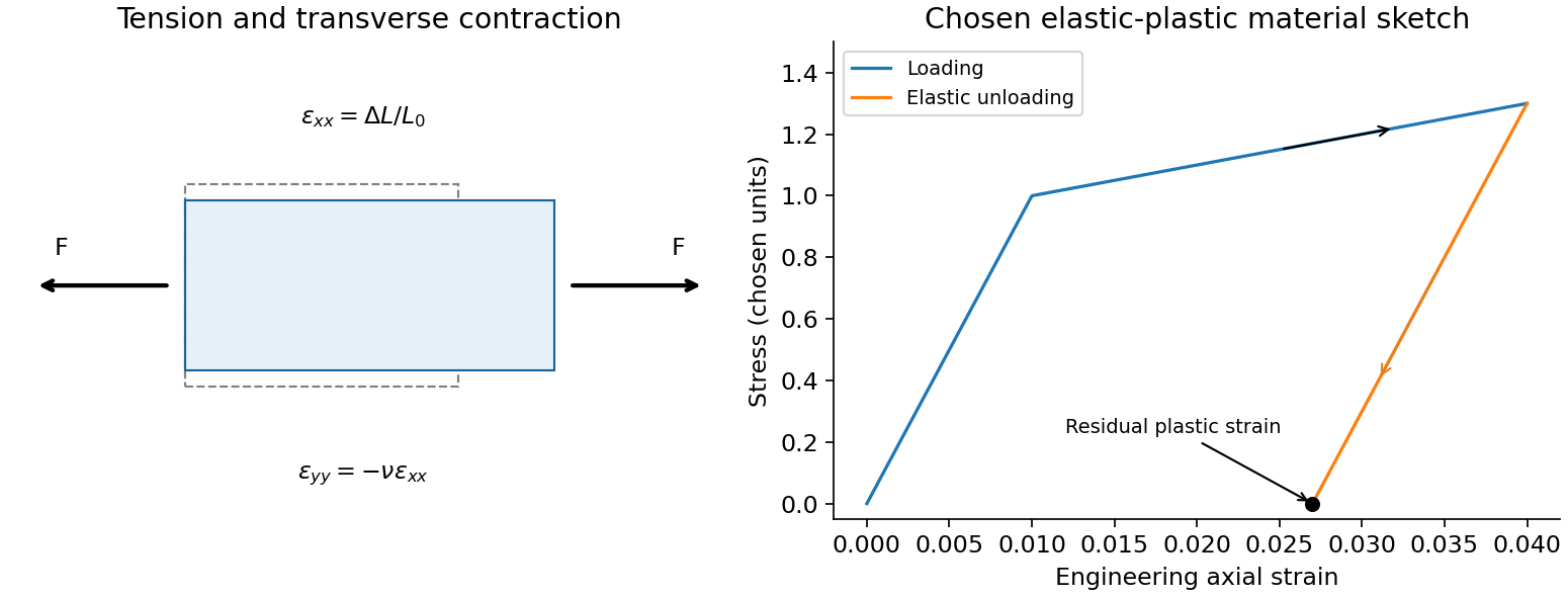
elastic deformation is recoverable on unloading; it need not remain linear at large strain. Beyond yield, irreversible rearrangements such as dislocation motion cause plastic strain, often followed by hardening. Ductile samples can neck before fracture; brittle failure has much less plastic deformation. Engineering stress uses initial area, while true stress uses the changing instantaneous area. A decreasing engineering stress during necking therefore need not mean that local true stress decreases. stress concentrations, flaws and loading geometry can determine failure before a uniform-material strength is reached. Viscoelastic materials also show rate dependence, creep and stress relaxation; their losses cannot be described by a static Hooke law alone.

A tensile test should measure force and gauge-length extension independently, correct machine compliance, align the grips, and control strain rate and temperature. Unloading distinguishes recoverable strain from a residual plastic extension. Separate shear or hydrostatic tests determine moduli that one axial measurement does not fix. Compression specimens need friction and buckling checks. Work per volume is $\int {\sigma }_{ij}d{ϵ}_{ij}$; the recoverable part is elastic energy, while a dissipative cycle produces a loss rather than creating energy. The original loading/unloading curve below is a chosen constitutive sketch, not measured material data.

At fixed positive pressure, the extrapolated term $C_{mp}\ln (T/T_0)$ tends to $-\infty$ as $T\to 0^{+}$. That prediction is not physically realistic for an equilibrium sample. The classical ideal-gas description with constant heat capacity cannot extend unchanged to absolute zero. A real substance generally undergoes phase changes, and quantum statistics and thermal freeze-out change its heat capacity and entropy. For a nondegenerate equilibrium ground state, the third law gives entropy approaching zero; residual ground-state degeneracy can give a finite residual value rather than this negative divergence. This is a breakdown of the extrapolation, not a violation of the third law by a real gas.

At fixed positive temperature, $-R\ln (p/p_0)$ tends to $+\infty$ as $p\to 0^{+}$. This is a physically meaningful unbounded-volume limit for a fixed mole number: $V_m=RT/p\to \infty$, so the number of accessible translational configurations grows without bound. For an ideal gas the entropy difference is $R\ln (V_{m,2}/V_{m,1})$ at fixed temperature. No finite vessel reaches an infinite entropy, and $p=0$ at finite temperature is not a finite-volume one-mole state. The divergence is approached by dilution; it does not conflict with the third law, which concerns a different temperature limit.

The microscopic magnetic response becomes a macroscopic field problem through the magnetization $\mathbf{M}$, the magnetic dipole moment per unit volume. Definein magnetostatics. Bound currents are represented by ${\mathbf{J}}_b=\nabla \times \mathbf{M}$ and surface current ${\mathbf{K}}_b=\mathbf{M}\times \hat{\mathbf{n}}$. Normal $B$ is continuous across an interface, while $\hat{\mathbf{n}}\times ({\mathbf{H}}_2-{\mathbf{H}}_1)={\mathbf{K}}_{\mathrm{free}}$. It is generally incorrect to impose continuity of every component of both fields. A linear isotropic material has $\mathbf{M}=\chi \mathbf{H}$ and ${\mu }_r=1+\chi$, but a ferromagnet usually requires a nonlinear, history-dependent constitutive relation.

Internal field differs from externally applied field. For uniform magnetization along a principal axis of an ellipsoid, the demagnetizing field is $-N_{d}M$ and $H_{\mathrm{int}}=H_{\mathrm{applied}}-N_{d}M$. A linear specimen therefore has apparent susceptibility $\chi /(1+N_d\chi )$ relative to the applied field. Shape is especially important for large susceptibility. A long closed magnetic circuit reduces stray fields; a bar magnet still has demagnetizing fields despite the absence of magnetic monopoles. Equivalent magnetic-pole descriptions are bookkeeping for magnetization divergence, not free magnetic charge.^[ref]

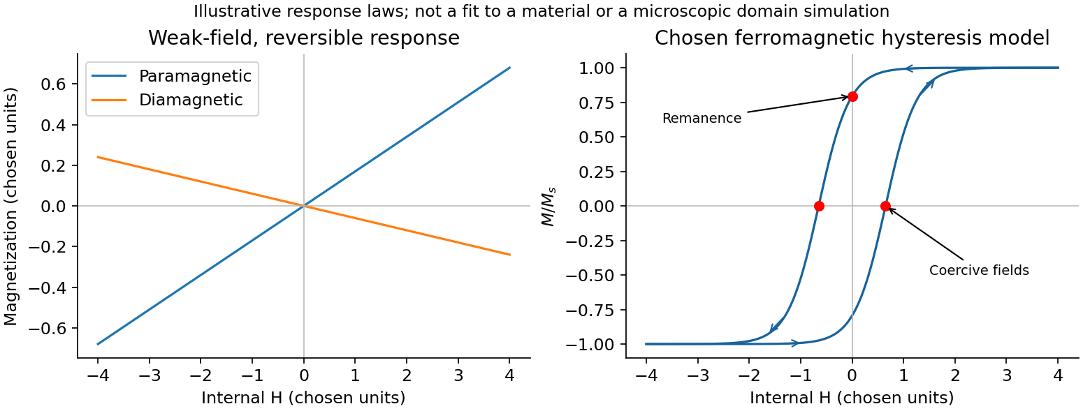
In paramagnetism, permanent localized moments are preferentially aligned by the field, against thermal disorder. For independent spin-one-half moments with projections $\pm \mu$, the two Zeeman energies givein the dilute weak-field limit with $B\simeq {\mu }_{0}H$. This is a Curie law; the response saturates at $n\mu$ when alignment dominates. More generally, spin $J$ gives $\chi ={\mu }_{0}n(g{\mu }_B{)}^{2}J(J+1)/(3k_{B}T)$. Interactions can produce a Curie–Weiss response $C/(T-\Theta )$ over a suitable range. Conduction-electron Pauli paramagnetism need not show the localized-moment $1/T$ law.

In diamagnetism, the field induces a magnetic moment opposing it, so the linear susceptibility is negative. The microscopic cause is the change in orbital electronic motion, and a closed-shell insulating material has no permanent atomic moment to orient. This weak response is often only mildly temperature dependent away from other transitions. It also exists as a background in materials with a stronger positive response. Perfect flux expulsion in a superconductor is a distinct collective phenomenon and should not be identified with ordinary weak atomic diamagnetism.

In ferromagnetism, exchange interactions stabilize spontaneous magnetic order below the Curie temperature. A specimen can have zero net moment while its magnetic domains remain locally magnetized in different directions. Domain-wall motion and moment rotation produce a large response; anisotropy and pinning lead to remanence, coercivity and hysteresis. Increasing field eventually approaches saturation. Heating above the ordering transition removes spontaneous order, although an applied field still induces a response. Soft magnetic cores favor easy reversal and small cyclic loss; hard permanent-magnet materials favor retained magnetization and resistance to reversal. These properties concern collective order and barriers, not merely independent moments all following a weak field.^[ref]

A practical distinction requires a controlled field sweep and a separate magnetic readout. A toroidal core with drive winding $N_1$, path length $l$ and current $I$ has approximately $H=N_{1}I/l$. A pickup winding measures ${\mathcal{E}}_2=-N_{2}AdB/dt$; integrating after calibration gives $B$, and $M=B/{\mu }_0-H$. Reversing the sweep reveals a loop whose positive loss area per volume is $\oint HdB$. An air-core/empty-holder reference, known geometry and turn count, offset correction, temperature control and slower sweeps test background, heating and rate-dependent eddy-current losses. A single force or susceptibility reading cannot establish spontaneous order or hysteresis. The original curves below are illustrative responses, not measured material data.