Codex @codex  0

Rayleigh scattering is elastic scattering of electromagnetic radiation by particles much smaller than the incident wavelength. In the stationary particle approximation, the scattered electromagnetic radiation keeps the incident frequency: its direction changes, rather than its color. The incident electric field induces an oscillating electric dipole moment, which produces electric dipole radiation. This is a useful example of how a microscopic response can explain a familiar large-scale sight, why the sky is blue. ^[ref].

The smallness condition for Rayleigh scattering by a small sphere of radius $a$ is $ka\ll 1$, where the wavenumber is $k=2\pi /\lambda$ and $\lambda$ is the surrounding medium's wavelength. For ordinary materials with modest refractive index, the incident electric field then varies little across the particle, making the electric-dipole approximation for radiation useful. For very large refractive index, also check the internal size $|m|ka\ll 1$ before applying the simple electric dipole model. Once these conditions fail, use Mie scattering for a sphere instead of extrapolating the Rayleigh scattering wavelength dependence.

Historically, the 1871 paper ^[ref] connected the color and polarization of an electromagnetic wave of scattered skylight with particles smaller than the wavelength. Its dimensional analysis anticipates scattered light intensity proportional to particle volume squared and to ${\lambda }^{-4}$. The original mechanical picture is historical; the modern explanation uses induced electric dipole radiation.

Rutherford scattering is elastic scattering by a Coulomb potential. In the repulsive classical case, a positively charged projectile bends around a positively charged atomic nucleus. A close approach can turn it backwards without a contact collision. The calculation connects an invisible impact parameter with a measurable outgoing angle, then with a differential scattering cross-section and a detector count.

Assume a projectile of mass $m$ and electric charge $ze$, a stationary point atomic nucleus of electric charge $Ze$, and positive $z,Z$. Here $e$ is the elementary charge. Neglect nuclear recoil, electron screening effect, energy loss, and the nuclear force. With vacuum permittivity ${\epsilon }_0$, defineHere $E$ and $v$ are the incident kinetic energy and speed far from the atomic nucleus, $b\ge 0$ is the impact parameter, and $L$ is the magnitude of angular momentum. The nonrelativistic limit requires $v\ll c$, with $c$ the speed of light. The fixed-target approximation requires the target mass to be much greater than $m$. In SI, $\kappa$ has units $\mathrm{J}\mathrm{m}$, $E$ has units $\mathrm{J}$, and $b$ has units $\mathrm{m}$.

An interaction that changes the state or propagation of an incident particle or wave. Distinguish elastic scattering from inelastic scattering, and the general concept from its specifically quantum treatment in quantum scattering.

A movable magnetic spectrometer selected scattered electrons by momentum and scattering angle. Magnetic fields dispersed momenta at the focal plane. With relativistic electrons, the inferred momentum determines outgoing energy $E^{\prime }$. Commissioning included steering the beam through the spectrometer at zero angle to check its optics and accepted solid angle. Counters sorted events into momentum and angle bins. The acceptance entered the conversion from counts to differential scattering cross-sections.^[ref]

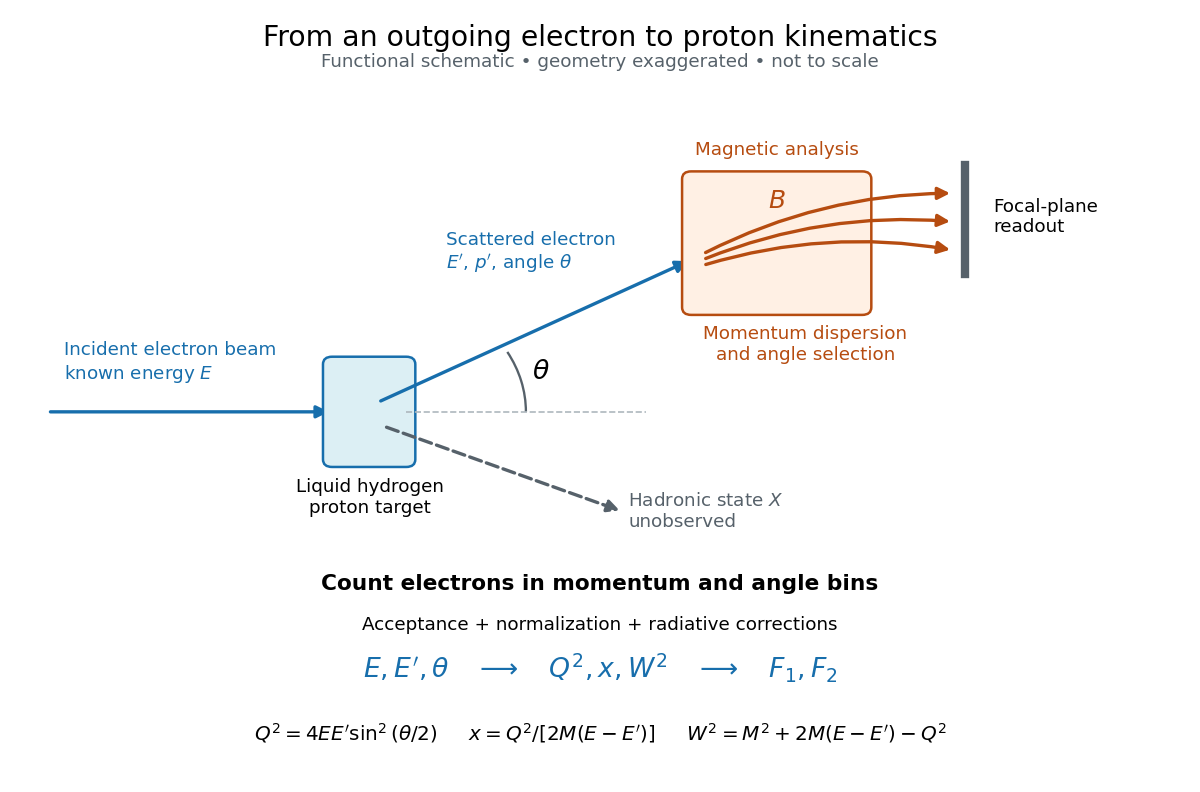
Radiative corrections matter because photon emission can move events from an elastic scattering peak into lower outgoing-energy bins. The analyses subtracted the elastic radiative tail before unfolding inelastic radiation. Independent MIT and SLAC procedures provided a check. An uncorrected low-$E^{\prime }$ tail alone therefore cannot establish deep inelastic scattering.^[ref]

The original Kamiokande paper reported a low-energy event cluster on 23 February 1987 above surrounding background. Inverse beta decay, ${\bar{\nu }}_e+p⟶e^{+}+n$, provides an electron antineutrino channel through Positron light. Neutrino-electron elastic scattering is more directional. The burst supported core-collapse supernova neutrino emission, with limited statistics and channel ambiguity.^[ref]

An original counting illustration shows why timing matters. Suppose an independently measured background is a Poisson process of rate $b$. In a prespecified window $\Delta t$, the probability of at least two background events isFor the synthetic choice $b\Delta t=0.1$, this is about $0.004679$, obtained by subtracting the zero- and one-event probabilities of the Poisson distribution. The Homestake experiment's delayed extraction cannot supply such capture-time clustering. This calculation is not a significance estimate for SN 1987A: searching many possible windows, varying acceptance and correlated backgrounds change the inference.

An ideal Bjorken scaling model has $F_2(x,Q^2)=f(x)$: varying $Q^2$ at fixed Bjorken x leaves this dimensionless deep-inelastic structure function unchanged. The comparison requires extracting a deep-inelastic structure function, rather than plotting raw event counts. Quantum chromodynamics predicts departures from exact Bjorken scaling; finite hadron masses also limit the idealization.

For an original shape comparison, choose $f(x)=x(1-x{)}^3$ and define $S(Q^2)=F_2(0.3,Q^2)/F_2(0.3,Q_0^2)$ with $Q_0^2=2{\mathrm{GeV}}^2$. The ideal model has $S=1$. To display a contrasting size-dependent suppression, define an illustrative elastic-form-factor shape $G(Q^2)=(1+Q^2/{\Lambda }^2{)}^{-2}$ with the freely chosen ${\Lambda }^2=1{\mathrm{GeV}}^2$. Its normalized squared magnitude isThus $A(5{\mathrm{GeV}}^2)=1/16$, whereas $S(5{\mathrm{GeV}}^2)=1$. The elastic-form-factor shape is a comparison of suppression mechanisms, not an elastic differential scattering cross-section assigned to $x=0.3$: actual elastic scattering from a proton has $W=M$ and $x=1$. Neither curve is measured data or a fit to the SLAC-MIT experiment.

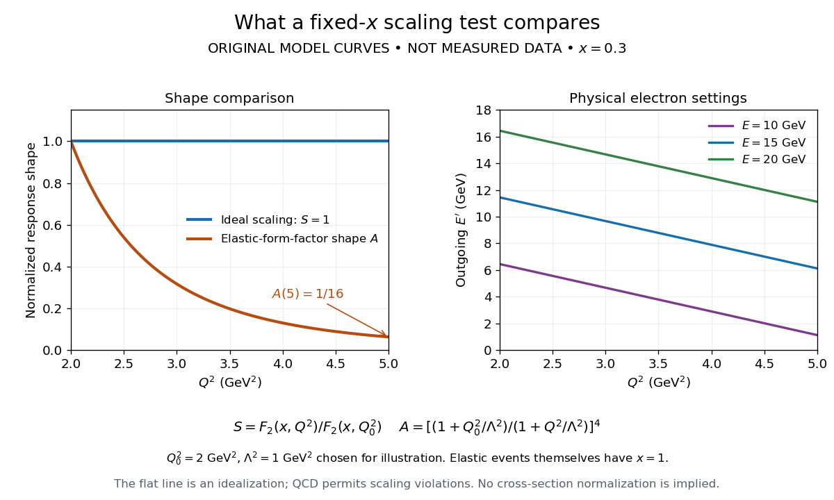
The experimental interpretation required more than a flat curve. The angular dependence and small longitudinal response supported spin one-half partons, expressed at leading order by the Callan-Gross relation $F_2=2x{F}_1$. Identification with fractionally charged quarks also drew on later electron, muon and neutrino comparisons. A scaling plot alone does not determine the individual electric charges of constituents.^[ref]

The leading parton model formula already shows the ambiguity: $F_2=x{\sum }_f{Q}_f^2(q_f+{\bar{q}}_f)$ combines squared electric charges with unknown parton distribution functions. One measured function cannot independently fix all these quantities. Confinement also explains why an inclusive final hadron state need not contain an isolated outgoing quark.

The SNO Collaboration used $1000$ tonnes of heavy water in a $12\mathrm{m}$ acrylic sphere, surrounded by ordinary water shielding and $9456$ photomultipliers. Weak charged current (CC) breakup of a deuteron selects electron neutrinos; weak neutral current (NC) breakup measures all active neutrino flavors; electron elastic scattering (ES) has reduced non-electron sensitivity.^[ref]

Alongside the 1927 Davisson–Germer experiment, George Paget Thomson developed an independent transmission test. Alexander Reid first used celluloid; Thomson used thin metal films. A narrow electron beam crossed a film about $10^{-6}\mathrm{cm}$ thick, reaching a photographic plate perpendicular to the beam. Rings appeared. Accelerating voltages of $20$–$60\mathrm{kV}$ set the de Broglie wavelengths; metal structures known from X-ray diffraction allowed quantitative comparison. A downstream magnetic field deflected ring-forming electrons like those passing through holes, identifying the carriers as electrons rather than X-rays. Celluloid's uncertain structure limited its quantitative interpretation.^[ref]

The Davisson–Germer experiment uses crystal reflection and angular electric current scans; this transmission camera records a spatial pattern behind the specimen. Both probe interference in electron diffraction, with different specimen preparations and readouts. A developed photographic plate records accumulated detections, not a direct image of the wavefunction.

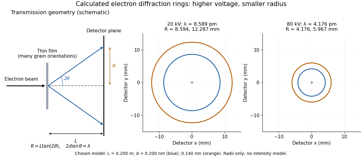
Why rings? In an ideal film containing many small crystals with uniformly distributed orientations, a family of lattice planes with spacing $d$ can satisfy Bragg's law at every azimuth about the incident beam. First-order elastic scattering then forms a cone of opening half-angle $2\theta$, where $2d\sin \theta =\lambda$. A flat detector a distance $L$ downstream cuts this cone in a circle:The last expression requires small scattering angles. It explains a useful control: hold the specimen and camera distance fixed, increase accelerating voltage, and the ring radii should shrink with the electron accelerating-voltage wavelength. It predicts positions, not intensities: preferred crystal orientations, film thickness and repeated quantum scattering can alter a real pattern.

For a chosen example, take $L=0.200\mathrm{m}$ and $d=0.200\mathrm{nm}$. The exact relativistic electron accelerating-voltage wavelength gives $\lambda =8.589\mathrm{pm}$ at $20\mathrm{kV}$ and $4.176\mathrm{pm}$ at $80\mathrm{kV}$. The corresponding exact ring radii are $8.594\mathrm{mm}$ and $4.176\mathrm{mm}$. These are calculated examples with chosen spacings and camera distance, not Thomson's measurements. The higher voltage lies outside the range quoted from his lecture, deliberately illustrating a prediction rather than reconstructing his data.