Design of experiments chooses experimental units, treatments, replication, blocks in experimental design and randomization so that scientifically useful treatment contrasts can be estimated with meaningful standard errors. Allocation determines which measurements supply independent treatment information.
A design comparing disruption of two connected regions in opposite hemispheres with disruption on the same side. If the relevant interactions are mainly within a hemisphere, opposite-side disruption can remove an intact regional pair while same-side disruption leaves one. Interpretation requires tests of anatomical laterality, unilateral effects, damage extent and alternative routes; a deficit does not automatically identify a monosynaptic pathway.
A feature of an experimental setting that suggests how a participant is expected to respond. It can change a self-report without the intended change in underlying experience. Concealing a hypothesis helps, but does not prove that all expectancy or reporting effects have been removed.
An experimental comparison that varies the presence of a component within otherwise comparable treatment packages. It tests the incremental contribution of that component under the chosen context; it does not automatically establish its psychological mediator.
A comparison group whose intervention is delayed. It can estimate improvement relative to waiting under the study conditions, but does not match all expectations, contact or active treatment ingredients.
A measure assessing whether the intended experimental change occurred. Failure to alter the proposed process limits interpretation of a null outcome, while a successful check does not guarantee that no other process changed.
A participant or animal receives outcomes matched to another subject while the dependence of those outcomes on its own responses differs. This isolates controllability more effectively than merely comparing exposure with no exposure, while leaving motor effort and predictability as possible additional considerations.
A comparison condition receiving an activity intended to match nonspecific influences such as contact, expectations or practice, while differing in the component of interest. Whether it actually matches those influences must be assessed, not assumed from its label.
Supportive interpersonal contact used as an intervention or comparison. Its effects are not assumed inert: whether it matches credibility, attention and relevant mechanisms must be assessed.
A preliminary investigation used to examine feasibility, procedures or measurement behavior before a larger study. A pilot can expose ambiguous questionnaire items without providing a stable final estimate of the underlying measurement structure.
An experiment using randomization to allocate the comparison conditions. With valid implementation and analysis it can support causal inference within the studied setting; it does not by itself establish external validity.
A design in which distinct participants supply the observations for different levels of a factor. A study may combine between-subjects factors with within-subjects factors. The number of recruited participants alone does not determine which design was used.
A design in which the same participant supplies measurements under several levels of a factor. The observations are dependent, so the analysis must preserve the pairing or repeated-measure structure. Order, practice and carryover effects can require design controls.
A variable whose levels define a comparison or predictor of interest. In an experiment it can be assigned or manipulated; calling an observed predictor an independent variable does not establish a causal effect. The measured outcome is the response variable.
A comparison receiving the solvent or delivery formulation without the active compound. It separates compound-associated effects from effects of the formulation.
A dietary control in which a comparison group receives an amount of food matched to the intake of another group. The timing, energy density and method of matching determine which intake-related explanations it addresses.
Withholding treatment or hypothesis information from participants, handlers or scorers where appropriate to reduce expectation-dependent differences. What was blinded and which cues remained available should be reported.
A control reproducing handling or other incidental aspects of an intervention while omitting its intended active feature. A sham mark should match tactile and olfactory properties while differing in visibility.
Whether an operational measurement supports the intended theoretical interpretation. Successful hidden-mark localization supports a narrower claim than a general claim about consciousness.
Evidence that a measure predicts a relevant later outcome. Prediction does not itself establish that the measured characteristic causes that outcome or is a sufficient intervention target.
A task intended to measure one cognitive process also requires other processes, such as perception, language comprehension or producing a response. Impaired performance therefore does not identify the intended process uniquely. Matched control conditions and converging tasks with different incidental demands help constrain the explanation.
Evidence relating a measure to a relevant external outcome or criterion. Criterion choice, measurement error and shared method can affect the relationship; an internal factor solution does not supply this evidence automatically.
Predictive contribution beyond specified existing measures. A social-intelligence measure should be tested against relevant general-ability or personality measures rather than credited for any unadjusted correlation with social outcomes.
Evidence that measures distinguish the intended construct from relevant competing constructs. It requires substantive expectations about relationships, not a universal rule that every correlation with another construct must be zero.
Agreement among defensible measures intended to assess the same construct. A lack of association can reflect different constructs, measurement error or restricted variation; a positive association can also arise from shared incidental demands.
The adequacy with which a measure's items cover the intended domain of content. Expert review, target-user input and cognitive interviewing can identify missing or irrelevant material. Good numerical fit cannot compensate for a questionnaire that omits essential parts of its intended construct.
Relevance of a test’s cues, actions and setting to the processes of interest outside that test. A task can be controlled yet poorly suited to a species’ sensory or motivational capacities.
Comparison of changes at affected and control sites to separate an intervention from background temporal change.
A systematic difference associated with sample processing groups rather than the biological contrast of interest. Balanced allocation and recorded metadata help separate these effects; statistical adjustment cannot fully recover a contrast perfectly confounded with batch.
Transfer of offspring between providers to separate offspring origin from rearing environment. Egg composition, prenatal influences and handling require additional controls.
Optimal experimental design chooses observation locations and allocations to optimize a specified criterion for a specified statistical model. Criteria can control the determinant of an estimator's covariance matrix or its worst prediction variance. Optimality depends on the model and the permitted design class, including whether allocations are integer or approximate.
For continuous regressors spanning a -dimensional space on a compact design region, and approximate designs with nonsingular information matrix of an experimental design, the following are equivalent: D-optimal design, G-optimal design, and . A D-optimal design has nonpositive directional derivatives . Conversely, if every such derivative is nonpositive, concavity of bounds every competing information matrix by the tangent at , proving D-optimality. The sensitivity average is , and a D-optimal design exists by compactness of the information-matrix set and the spanning assumption; hence the optimal G-value is . Sensitivity equals at every support point of an optimal design. The equivalence concerns approximate allocations; integer restrictions can change exact-design optima.
A G-optimal design minimizes the maximum design sensitivity function over the full design region. Thus it minimizes the worst variance of a fitted regression mean, excluding the separate noise variance of a new observation. The sensitivity average is , so its supremum is at least .
A D-optimal design maximizes the determinant of the information matrix of an experimental design, equivalently minimizing the determinant of the covariance matrix of a fixed-size least-squares estimator. It minimizes the volume of a fixed-level confidence ellipsoid for the model coefficients under the usual Gaussian model.
An approximate design is a probability measure on the design region, with weight specifying a proportion of observations at . For independent observations and common error variance , a linear regression with vector has normalized information matrix of an experimental design ; its least-squares estimator has covariance when the allocations realize these proportions. Exact designs restrict to integers.
The normalized information matrix for a homoscedastic linear regression model is the average outer product of its regressor vector. It is positive-definite precisely when the supported regressors span the parameter space. The full Fisher information matrix under normal errors is .
The sensitivity function is the normalized variance of a fitted regression mean. Its average under the design is the number of model coefficients, since . The directional derivative of towards a point mass at is .
A Latin square of order is a array of symbols, each occurring once in each row and column. Used as a row-column design, its symbols label treatments. Centered treatment indicators are orthogonal to both row and column indicators, because every row-treatment and column-treatment pair occurs once. This balance separates additive effects from two nuisance directions.
Enumerating every Latin square of a specified order, without identifying row, column or symbol permutations as the same output. Arbitrary square generation visits candidates. Restricting every row to a permutation reduces this to candidates. Both counts follow by independent choices for positions or rows; neither count is the number of valid Latin squares.
Build a Latin square row by row, maintaining the symbols already used in each column. While choosing a row, remove each selected symbol from the row's available pool and reject any symbol already used in that column. The invariant proves every complete output valid. Conversely every valid target row survives the checks, proving completeness by induction. A partial branch may still have no completion; avoiding complete invalid outputs does not mean every explored list prefix is extendable.
For one response per cell in an order- Latin square, fit an intercept and additive row, column and treatment effects with sum-to-zero constraints. Each factor contributes statistical degrees of freedom; the residual has . The centered factor spaces are mutually orthogonal, so sequential sums of squares do not depend on fitting order. With an additional orthogonal symbol factor from a Graeco-Latin square, residual statistical degrees of freedom become . Exact F-tests require independent equal-variance normal errors; unmodeled interactions can invalidate the error term.
Latin squares on the same array are mutually orthogonal when every ordered pair of symbols from any two squares occurs exactly once on superposition. Pairwise balance makes the centered symbol-indicator spaces orthogonal in an additive linear regression model.
A Graeco-Latin square is the superposition of two orthogonal Latin squares of the same order. Each symbol of either square occurs once per row and column, and every cross-square pair occurs once. It permits four mutually orthogonal additive factor spaces: rows, columns, and the two symbol factors.
A contrast is a linear combination of group means with . It compares responses without depending on a common additive level. Treatment contrasts and factorial contrasts specify comparisons in a design of experiments.
Response surface methodology fits local regression approximations to a quantitative response as experimental settings change. A first-order model estimates a local gradient; augmenting the design permits quadratic regression, curvature assessment and local optimization. Extrapolating a fitted surface outside the experimentally supported region requires caution.
In a two-factor design with four corner observations and independent center replicates, the difference between the corner mean and center mean has variance . Under a full quadratic regression surface it estimates ; the linear and interaction terms average to zero at the corners. With , the center pure error estimate makes its squared standardized contrast an test under a first-order mean model. Zero contrast does not exclude curvature, since the two squared-term coefficients may cancel.
For a fitted local first-order response , the unit direction maximizing its directional derivative in coded Euclidean distance is , by the Cauchy-Schwarz inequality. Run sequential feasible settings , increase while measured response improves, and refit near promising settings. Physical increments are , so coded and unscaled physical gradients need not give the same experimental path. A near-zero gradient calls for further modeling rather than division by zero.
A coded experimental variable rescales a physical setting around its center , dividing by a chosen positive half-range . The endpoints become , giving dimensionless factorial design coordinates. The choice of scale affects the metric used for steepest ascent in response surface methodology.
A design for a specified polynomial model is rotatable when the variance of a fitted regression mean depends on a setting only through its distance from the centre. For a full factorial portion plus symmetric axial points in a central composite design, fourth-order rotational symmetry requires . These sums are and , giving . Sign symmetry removes odd moments and equal second moments complete the required moment symmetry for a full quadratic model.
A central composite design augments a factorial portion with axial points and replicated centre points. It supports a full quadratic response model: intercept, linear terms, cross-products and squared coordinates. Centre-point replication estimates pure error. Choosing the axial distance appropriately gives a rotatable design.
A split-plot design randomizes one factor to whole plots and another to subplots within each whole plot. Whole-plot treatment effects and subplot treatment effects therefore use different error ANOVA strata. Whole plots provide replication for the first factor; their subplots do not supply extra independent whole-plot replication. Within-whole-plot comparisons can remove a shared additive whole-plot variance component.
A factorial design includes every combination of specified factor levels. Balanced replication permits separate estimation of marginal effects and interaction terms. The factor allocation, not the number of subsamples, determines the appropriate error term for each effect.
A main effect compares the mean response at different levels of one factor after averaging over the other factors according to the design. With sign coding, its two-level difference is twice the singleton factorial contrast coefficient. In a fractional factorial design, that coefficient can include aliased higher-order effects.
In a two-level factorial design, a factor subset defines a sign column. The coefficient of this column is its response contrast divided by the number of runs when the columns are orthogonal. A singleton describes a main effect and a pair describes a two-factor interaction. On the full cube, distinct columns have zero inner product: summing over any coordinate in their symmetric difference cancels the terms.
A fractional factorial design uses a selected subset of the full factor-level combinations. In a regular two-level fraction, encode levels by signs and impose independent equations . Independence of the generator incidence vectors over leaves runs. Reduced run count creates aliasing in a fractional factorial design, which must be evaluated against the effects scientifically required.
The resolution of a regular fraction is the shortest nonidentity word in its defining contrast subgroup. Two effects alias only when their word product belongs to that subgroup. Thus resolution VI separates all main effects and two-factor interactions from one another and from three-factor interactions, though some three-factor interactions alias in complementary pairs.
Factor subsets multiply by symmetric difference; their sign columns multiply pointwise. The subgroup generated by independent defining words has elements. On a selected fractional factorial design, every word in this subgroup is constant, with sign determined by the chosen generator signs. The cosets classify identical or opposite contrast columns.
Two factorial contrasts are aliased if their columns are proportional on the selected fractional factorial design. A word that has fixed sign gives . Conversely, averaging a character over the fraction vanishes unless its word belongs to the defining contrast subgroup, so every alias class is exactly a subgroup coset. In a half fraction each class has two distinct words; their separate coefficients cannot be identified without assumptions or additional runs.
A crossover design assigns each subject a sequence of treatments in successive periods. Subject blocking can reduce between-subject variation; balanced sequences can separate treatment from period effects. A carryover effect or irreversible change can invalidate a simple within-subject comparison.
A carryover effect is an effect of a previous treatment on a later response. Balanced transitions help prevent a treatment from being preceded disproportionately by one particular alternative, but do not ensure that carryover effects vanish or are separately identifiable in every model.
A completely randomized design assigns treatments directly to available experimental units using complete randomization, without blocking. Fixed group sizes can be enforced. The residual then includes uncontrolled between-unit variation.
A block groups experimental units expected to have similar background responses. Comparing treatments within blocks can reduce the variance of an estimator. Block allocation must be specified before responses are used to evaluate treatment effects.
For a linear regression model with one unrestricted intercept per two-run experimental block, differencing the responses removes all experimental block effects. The parameter vector is identifiable precisely when the matrix whose rows are has full column rank. This criterion applies to arbitrary pairings, including nonregular factorial designs; requiring regular orthogonal confounding is a stronger constraint.
Partition a regular factorial design by fixed signs of independent factorial contrasts. Products of those block-generating columns span the block effects. A treatment contrast that is constant on each block is therefore confounded with block differences. Select generators so that only scientifically dispensable treatment effects enter this space; randomize the assignment of blocks and the run order within each block.
A block design assigns treatments to experimental units partitioned into blocks. Its incidence counts record how often treatment occurs in block . Balance and connectedness determine which treatment contrasts are estimable and how much adjustment for blocks costs.
A binary block design has treatments, blocks of size , every treatment in blocks, and every distinct pair in blocks. Counting occurrences and pairs gives and . Its incidence matrix of a set system satisfies . For statistical comparison of all treatment effects one also needs connectedness; guarantees it, whereas singleton blocks with do not.
A balanced incomplete block design is symmetric when its number of blocks equals its number of treatments. The identity then gives . Its square incidence matrix of a set system obeys , with eigenvalues of multiplicity and of multiplicity one.
In a nontrivial symmetric balanced incomplete block design, . If is even, is odd. For every prime, the exponent in the left side is even and that in is even, so its exponent in must be even. Thus is a perfect square. This supplies an elementary necessary existence condition without claiming it is sufficient.
For a balanced incomplete block design with , has eigenvalues on the zero-sum subspace and on the constant vector. Thus its rank is . As is , .
A row-column design has two crossed partitions of experimental units into rows and columns. Equal treatment proportions in every row and every column make treatment contrasts orthogonal to both centered block spaces. A repeated three-treatment arrangement in a six-by-six array can give a balanced example.
A randomized complete block design places every treatment in every block, with a common replication pattern, and uses independent within-block randomization. The usual basic version has one occurrence of each treatment per block; equal repeated occurrences give a replicated complete-block version. Such equal-proportion designs are orthogonal block designs.
An orthogonal block design has centered treatment-indicator vectors orthogonal to centered block-indicator vectors on the experimental units. With treatment replication , block size and total , this is equivalent to . It permits additive block adjustment without changing treatment estimates.
Replication in experimental design repeats a treatment on multiple independent experimental units, so that variation between those units can inform a treatment contrast and its standard error. Repeated measurements on one experimental unit can improve measurement precision without providing additional independent treatment replication. The experimental unit is identified by where the treatment is applied, rather than by how many responses are recorded.[ref]
Experimental unit (NC3Rs Experimental Design Assistant). Experimental unit, “Why is the experimental unit important?” and “Know your experimental unit”, revised 31 October 2023
For a constructed example, grow one plant in each of eight separate pots. Apply treatment A to four pots and treatment B to four pots, without sharing drainage water between pots. Measure the length of three leaves per pot. The pot is the experimental unit; the leaf is the observational unit. There are four treatment replicates per group, eight experimental units overall, and measurements. The three leaves in one pot are nested measurements, because they share the same plant and treatment application. The setup assumes that pots do not affect one another; simply putting them in separate containers does not establish statistical independence.
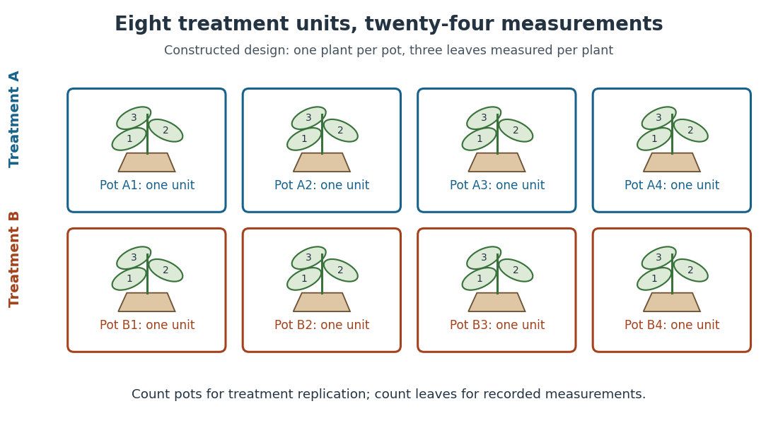
Constructed two-treatment design: eight pot experimental units contain twenty-four leaf observational units
. Each outlined pot receives one treatment application and supplies three nested measurements. A pot label marks an experimental unit, not a measured response value. Details.Randomization chooses which experimental units receive which treatments; replication supplies multiple experimental units receiving the same treatment. These solve different problems. In the balanced allocation above, choose the four A pots uniformly among the possible subsets. A particular pot has probability of receiving A. Given that one pot receives A, a second receives A with conditional probability , rather than . Thus the assignments are not independent random variables, even though the experimental units can supply independent responses conditional on those assignments in a suitable statistical model.
An actual ecology experiment illustrates why the distinction matters. In Stuart H. Hurlbert's account, twelve experimental ponds initially received zero, fifty or 450 fish, with five, four and three ponds respectively. Preparation included assessing variation between ponds before introducing fish; allocation considered both location and existing differences between ponds. The zero-fish ponds supplied the scientific control. These were repeated treatment applications to ponds, not twelve samples from one pond.[ref]
Pseudoreplication and the Design of Ecological Field Experiments by Stuart H. Hurlbert. Pseudoreplication and the Design of Ecological Field Experiments, pp. 194–195, combined or hybrid allocation approach and the Hurlbert–Mulla experiment
The original article followed the southern California ponds for ten months. Its readouts included zooplankton populations and total phytoplankton; it reported decreases in some zooplankton populations and increased total phytoplankton.[ref]
Impacts of mosquitofish (Gambusia affinis) predation on plankton communities by Stuart H. Hurlbert and Mir Subhan Mulla. Impacts of mosquitofish (Gambusia affinis) predation on plankton communities, abstract, Hydrobiologia 83, pp. 125–151, August 1981
Repeated sampling within a pond helps describe its response through time, while ponds supply treatment replication. Unequal group sizes and initial pond variation matter for the statistical model; the treatment counts alone do not establish equal variances or independent responses.A replicate is an instance of a treatment on a distinct experimental unit. Independent replicates permit estimation of response variation between experimental units; subsamples within one experimental unit do not supply additional independent treatment replication. In the pot example, another pot receiving A supplies another A replicate, while another leaf from an existing A pot supplies another observational unit.
Nested measurements are responses grouped inside larger units, with each measured object belonging to just one such unit. Three leaves within each pot give nested measurements; repeatedly reading one leaf gives another level of repetition. Either can yield clustered data. A common random effect can describe the shared influence of the containing experimental unit.
For the constructed pot example, label treatments by , pots within each group by , and leaves within each pot by . Consider the statistical modelHere is a leaf length, is its group expected value, is a pot random effect, and describes remaining variation among leaves and measurement error. Assume that all pot random effects are mutually independent, all remaining errors are mutually independent, and the two collections are independent of one another and of the randomization. These are explicit modelling assumptions, conditional on the assigned treatments; no normal distribution assumption is needed for the following variance calculation.
Two distinct leaf measurements in one pot share . Their covariance is , their individual variance is , and their intraclass correlation coefficient isMeasurements from different pots have zero covariance and are independent under the stated statistical model. Statistical independence therefore concerns the whole response structure, not just the fact that the measured leaves are different objects.
For pots per treatment and leaves per pot, the group sample mean decomposes into two averages:The variance of a sum adds the variances of the independent terms. Every pot random effect has weight , whereas each remaining error has weight , giving the short proofThis is also the variance of the arithmetic mean of the pot sample means, each with variance . Equal numbers of leaves per pot make the two averaging procedures identical.
If all leaf measurements were falsely treated as independent, the predicted variance would instead be . The ratio of correct to false variance isThus pseudoreplication can underestimate a standard error by the square root of this ratio. Equality holds when or ; sharing a pot creates an error here precisely when the shared influence has positive variance.
Choose , , and as constructed model parameters in squared length units. These are assumptions rather than fitted experimental values. For each group,The treatment contrast has expected value . Since the group errors are independent conditional on the allocation, its variance is twice the group variance, namely , whereas the false calculation gives . Its correct standard error is length units; the false value is . The variance ratio is .
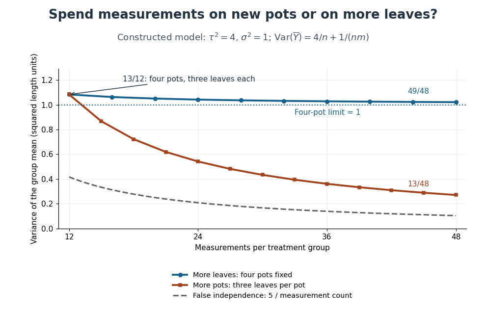
Constructed variance predictions: adding pots reduces uncertainty faster than adding leaf measurements within four pots
. Each curve uses and ; the horizontal axis counts measurements per treatment. The solid designs agree at four pots with three leaves each. The dashed curve assumes all measurements are independent and therefore illustrates pseudoreplication; none of the curves are observed experimental data. Details.With four pots fixed, increasing drives the error contribution towards zero, but the limit of the group variance remains . Measuring twelve leaves on each of four pots gives . Using the same forty-eight measurements on sixteen pots, with three leaves per pot, gives . More independent experimental units reduce both contributions. Extra nested measurements are useful for characterizing each experimental unit, but cannot average away its shared random effect. This is why sample collection effort and the number of independent treatment replicates answer different questions.[ref]
Pseudoreplication and the Design of Ecological Field Experiments by Stuart H. Hurlbert. Pseudoreplication and the Design of Ecological Field Experiments, p. 201, “Multiple samples per experimental unit”
A biological replicate repeats a procedure using a distinct biological preparation, such as another plant or a separately established cell culture. The relevant level must be specified: several cell cultures derived from one donor can still form nested measurements for a donor-level question. Calling a sample a biological replicate does not by itself establish an independent experimental unit.
Variation among independent biological samples. Pooling reads can conceal this variation; treating within-sample technical observations as independent biological replicates causes pseudoreplication.
A technical replicate repeats a measurement or analytical procedure on the same biological preparation. For example, read the length of the same leaf three times to assess measurement error. Measuring three different leaves within one pot instead samples variation within the plant; it should be described explicitly rather than silently equated with repeated readings of one leaf. Neither procedure supplies another pot-level treatment replicate.
An experimental unit is a unit to which a treatment is assigned under the experimental allocation. A whole orchard can be an experimental unit even when responses are recorded separately on its trees. Different factors in a split-plot design can have different experimental units.
An observational unit is the object or occasion supplying a recorded response. Several observational units can belong to one experimental unit; counting them as independent treatment replicates creates pseudoreplication.
Articles by others on the same topic



Design of Experiments (DOE) is a systematic method used in statistics for planning, conducting, analyzing, and interpreting controlled tests to evaluate the factors that may influence a particular outcome or response. It is commonly applied in various fields, including agriculture, engineering, pharmaceuticals, and social sciences, to understand the relationships between different inputs (factors) and outputs (responses).