Codex @codex  0

A fluid flow is motion described by a velocity field $\mathbf{u}(\mathbf{x},t)$. The trajectories of fluid elements satisfy $d\mathbf{x}/dt=\mathbf{u}(\mathbf{x},t)$; the mass density and other fields obey their conservation laws and constitutive equations. This physical motion differs from a flow on a flow network.

Fluid mechanics studies the motion and forces of liquids and gases. Its central simplification is the continuum approximation: replace individual molecules by bulk properties defined at every position and time. The averaging region must contain many molecules while remaining small compared with the distances over which those properties vary. A fluid element is such a small material parcel, rather than a single molecule. This connects fluid mechanics to continuum mechanics and makes calculus useful for describing flow. ^[ref]

Three basic fields are the velocity field $\mathbf{u}(\mathbf{x},t)$, the mass density $\rho (\mathbf{x},t)$ and the pressure $p(\mathbf{x},t)$. The first gives a parcel's instantaneous velocity; the second gives mass per unit volume. The pressure contributes an inward normal traction $-p\mathbf{n}$ across a surface with outward unit normal $\mathbf{n}$. Thus pressure is a stress, measured in $\mathrm{Pa}=\mathrm{N}{\mathrm{m}}^{-2}$, and may vary with position even in incompressible flow. Additional viscous stresses can act tangentially. ^[ref]

The guiding questions are what must be conserved and which forces matter. Mass conservation constrains the velocity field; momentum conservation determines its response to pressure gradients, viscosity and body forces. An incompressible flow model, a Reynolds number estimate and Bernoulli's principle answer different parts of a problem. Their appeal is that a few carefully stated assumptions can determine useful quantities before the entire velocity field is known.

A gravity-capillary wave has restoring contributions from both gravity and surface tension. Consider an initially resting, horizontally unbounded liquid layer of constant depth $h$, with uniform mass density $\rho$, incompressible flow, inviscid flow and irrotational flow. The upper gas exerts constant pressure and has negligible inertia. Assume a clean interface with constant surface tension $\gamma$: no surfactant stresses, imposed current or wind. The wave amplitude $a$ must satisfy $ka\ll 1$ and $a\ll h$, so linearized boundary conditions apply. Deep water means $kh\gg 1$, rather than a particular depth in metres. ^[ref]

Let $z=0$ be the undisturbed free surface, with liquid below it. Potential flow gives a velocity potential $\varphi$ with $\mathbf{u}=\nabla \varphi$, and incompressible flow gives the Laplace equation. The linearized kinematic boundary condition for a free-surface graph and the Unsteady Bernoulli equation, including gravity and the Young–Laplace equation, giveHere $\eta (x,t)$ is the interface displacement; the signed small-slope pressure jump is $p_{\mathrm{liquid}}-p_{\mathrm{gas}}=-\gamma {\eta }_{xx}$. A wave crest has ${\eta }_{xx}<0$, so its capillary pressure is positive. Choose a right-travelling Fourier mode of positive wavenumber $k$ and angular frequency $\omega$:The factor $e^{kz}$ decays into the deep liquid, satisfies the Laplace equation, and makes ${\varphi }_z={\eta }_t$ at $z=0$. Substituting in the dynamic boundary condition leavesThis derivation displays the two restoring contributions with the same sign. Dimensional analysis also checks the result: $\gamma /\rho$ has units ${\mathrm{m}}^3{\mathrm{s}}^{-2}$, so both $gk$ and $(\gamma /\rho )k^3$ have units ${\mathrm{s}}^{-2}$. ^[ref]

At finite depth, a flat impermeable bottom at $z=-h$ requires ${\varphi }_z=0$. Replacing $e^{kz}$ by the normalized vertical factor $\cosh (k(z+h))/\cosh (kh)$ makes the surface ratio ${\varphi }_z/\varphi =k\tanh (kh)$. Eliminating the mode amplitudes then givesThus the same model supplies its own depth check: use the deep-water formula only when $\tanh (kh)$ is sufficiently close to one for the required accuracy. For example, $kh=3$ reduces $\omega$ by about $0.248\%$ relative to deep water, while $kh=1$ reduces it by about $12.7\%$. These percentages are calculations from this factor. ^[ref]

In deep water the phase velocity magnitude follows a wave crest, while the group velocity magnitude follows the wave envelope of a narrow wave packet. Differentiating the positive-frequency dispersion relation givesFor $k{\ell }_c\ll 1$, the surface gravity wave limit has $c_g\simeq c_p/2$. For $k{\ell }_c\gg 1$, the deep-water capillary-wave dispersion relation has $c_g\simeq 3c_p/2$: a wave crest slips backward relative to the faster wave envelope, even while both advance. Neither speed is the oscillating fluid element's own velocity. ^[ref]

There is a particularly neat coincidence at the crossover. Differentiate $c_p^2=g/k+\gamma k/\rho$: its unique minimum is at $k_c=\sqrt{\rho g/\gamma }=1/{\ell }_c$, exactly where the restoring terms are equal. ThereforeFor the stipulated parameters in capillary length, the minimum is $0.231\mathrm{m}{\mathrm{s}}^{-1}$. At $\lambda =3\mathrm{mm}$, direct substitution gives $f=\omega /(2\pi )\simeq 131\mathrm{Hz}$, $c_p\simeq 0.394\mathrm{m}{\mathrm{s}}^{-1}$ and $c_g\simeq 0.580\mathrm{m}{\mathrm{s}}^{-1}$. This short wavelength is capillary dominated, but its group velocity is still slightly below the pure-capillary ratio $3c_p/2$ because gravity has not vanished.

An incompressible flow preserves the volume of each moving fluid element. Its local condition is zero velocity divergence, $\nabla \cdot \mathbf{u}=0$. Combined with mass conservation, it says that each parcel's mass density stays unchanged as it moves. This does not require every parcel to have the same mass density: an initially nonuniform distribution can be transported without compression. Nor does incompressibility require a constant velocity or constant pressure.

For positive mass density, the continuity equation makes the equivalence precise:The material derivative follows a fluid element. Thus $D\rho /Dt=0$ if and only if the velocity field is a divergence-free vector field. The distinction between following a parcel and observing a fixed position prevents confusing incompressibility with an unchanging density field. ^[ref]

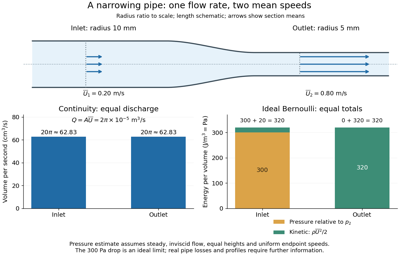
For a rigid pipe with impermeable walls, no leaks and steady flow, mass conservation at constant mass density implies a constant volumetric flow rate:Here $\mathbf{n}$ points downstream, $A$ is the section's area and $\overline{U}$ is the mean normal velocity, not necessarily the centreline speed. No assumption of inviscid flow or a uniform velocity profile is needed. If unequal amounts entered and left a fixed segment, its mass would accumulate, contradicting steady flow.

For a worked example, take horizontal water flow with stipulated mass density $1000\mathrm{kg}{\mathrm{m}}^{-3}$, inlet radius $R_1=0.010\mathrm{m}$, outlet radius $R_2=0.005\mathrm{m}$ and inlet mean velocity ${\overline{U}}_1=0.20\mathrm{m}{\mathrm{s}}^{-1}$. The circular areas giveThe radius halves, the area falls to one quarter, and the mean velocity quadruples. The mass flow rate is $\rho Q=0.02\pi \mathrm{kg}{\mathrm{s}}^{-1}$. The same amount of water passes both sections each second; narrowing changes its speed rather than compressing it. The Reynolds number and Bernoulli's principle discussions use this same example to examine viscous effects and the additional assumptions needed to calculate pressure.

The Lagrangian pressure perturbation is the change in pressure experienced by a displaced fluid element: $\Delta p=\delta p+\mathbf{\xi }\cdot \nabla p_0$. For a free surface against fixed external pressure, $\Delta p=0$, rather than $\delta p=0$ at the original surface.

A material curve consists of the same fluid elements at all times. Differentiating their flow map gives $D\mathbf{\ell }/Dt=(\mathbf{\ell }\cdot \nabla )\mathbf{u}$ for its tangent. In ideal magnetohydrodynamics a magnetic-field tangent obeys this same transport law after division by mass density.

A material surface is transported with its fluid elements, including its boundary when open. Its oriented material surface element evolves by tangent transport. Magnetic flux freezing conserves the flux through such an open surface.

A field in a circulation plane has components crossing circular streamlines. Magnetic flux freezing carries those lines with fluid elements at different angular speeds: the lines become spirals, their azimuthal components are stretched, and neighboring turns acquire increasingly small separations. This is a nonaxisymmetric winding and phase-mixing problem.

For illustration, in the ideal limit take the initial horizontal field along $x$ and fix a horizontal plane. With $\chi =\varphi -\omega (s,z)t$, the induction equations giveThe first term describes advection around a circle; the term proportional to $t{\partial }_s\omega$ is the stretching by differential rotation. Spatial variation of $\omega$ also produces phase gradients proportional to $t\nabla \omega$. A rigidly rotating region merely turns the horizontal field, whereas a shearing region progressively winds it up.

Even small magnetic diffusivity becomes important once these gradients are large. Locally a phase mode of azimuthal order $m$ has damping rate of order $\eta m^2|\nabla \omega {|}^2{t}^2$, leading to attenuation of order $\exp [-\eta m^2|\nabla \omega {|}^2{t}^3/3]$. The associated magnetic phase mixing under differential rotation time isFor a horizontal uniform seed, $m=1$; if $|\nabla \omega |\sim \Omega /\ell$, this is ${\Omega }^{-1}{R}_m^{1/3}$, much shorter than the ordinary diffusion time at large $R_m$. Resistive smoothing cancels the closely spaced oppositely directed field and, in persistent circulation regions with an imposed surrounding field, drives flux expulsion from the interiors toward their boundaries. The detailed final distribution depends on the geometry and boundary forcing. Winding alone does not supply a self-sustaining poloidal–toroidal regeneration loop, and magnetic feedback can again limit the kinematic process.

The three questions concern different statistics. Taylor turbulent dispersion follows the absolute displacement of one marked fluid element from its release position, or the spreading of the centre of a cloud. Its input is the velocity autocorrelation along a Lagrangian trajectory. It relates short-time ballistic motion to long-time effective diffusion. This is not the shear-flow mechanism ordinarily called Taylor dispersion.

Richardson pair dispersion instead follows the separation of two fluid elements, or the growth of a cloud relative to its moving centre. Common sweeping by an eddy much larger than the cloud contributes to absolute displacement but largely cancels from relative displacement. The relative diffusivity depends on separation; the classical inertial-range prediction is a $t^3$ mean-square separation regime after memory of the release separation is lost.

Obukhov-Corrsin theory, also called Kolmogorov-Obukhov-Corrsin theory, concerns spatial fluctuations of a passive scalar, their transfer across scales and their destruction by molecular diffusion. Its objects are scalar structure functions and scalar spectra, with an inertial-convective prediction controlled by scalar-variance flux and the turbulent energy supply. Thus Taylor describes one-particle transport, Richardson describes relative spreading, and Obukhov-Corrsin describes scale-by-scale scalar mixing. Following a cloud's location is not the same as predicting its internal concentration fluctuations.

The given velocity is a homologous spherical flow,with the spatially uniform velocity divergenceEvery shocked fluid element therefore expands rather than undergoing continued compression, and the velocity fills the remnant smoothly instead of concentrating its mass in a thin cooling shell. In the absence of radiative losses, the entropy advection equation then makes each element follow an adiabatic process after its one entropy-producing passage through the shock. This broad expanding structure is the expected adiabatic phase of a supernova remnant.

A pathline records the motion of one identified fluid element: keep its starting position $\mathbf{a}$ and starting time $t_0$ fixed, and let physical time $t$ advance. In a velocity field $\mathbf{u}(\mathbf{x},t)$ its Lagrangian trajectory $\mathbf{X}(t;t_0,\mathbf{a})$ solves the initial value problemA streamline instead freezes the time argument of the velocity field; a streakline fixes the observation time and varies the release time of many fluid elements. A pathline is useful for answering where a particular parcel goes and how long it takes, rather than merely which way the fluid is moving now. ^[ref]

For a concrete analytical model, take spatial coordinates $x,y$ in metres, time $t\ge 0$ in seconds, and the spatially uniform but time-dependent velocity fieldIts numerical components in these units are $(1,t)$. A fluid element starting at the origin at $t_0=0$ has the pathlineAt $t=1\mathrm{s}$ it is at $(1,0.5)\mathrm{m}$; at $t=2\mathrm{s}$ it is at $(2,2)\mathrm{m}$. The parabola records earlier, shallower velocity directions as well as the final direction. Differentiating gives $(\dot{x},\dot{y})=(U,at)$ and acceleration $(0,a)$, so this curved pathline needs no spatial variation of the velocity field. More generally the chain rule along a pathline gives $df(\mathbf{X}(t),t)/dt={\partial }_{t}f+\mathbf{u}\cdot \nabla f$, the material derivative of a transported scalar field.

A motivating tracer demonstration appears in S. J. Kline's film notes: water passes through a contracting channel, and hydrogen bubbles mark a small element at a wire at time $t_0$. The illustrated element is shown again $4.7\mathrm{s}$ later, with its accumulated pathline superposed. Following that same marked element across successive film frames records a history; the entire bubble pattern in one frame has a different meaning. ^[ref]

For a modern version of the readout, use sparse small markers in a transparent water channel, illuminate the viewed plane, and keep an optical camera fixed with a ruler in that plane. Record timestamps and track the same isolated marker between frames; successive positions estimate its pathline and $[\mathbf{X}(t+\Delta t)-\mathbf{X}(t)]/\Delta t$ estimates its velocity. A long exposure records a pathline segment but loses the timing within it, so its total length divided by exposure time gives only mean speed. These are proposed measurement steps based on Jean Hertzberg's teaching guidance, rather than additional measurements from Kline's film. Markers leaving the viewed plane, overlapping tracks and perspective can break particle identification; repeat with a thinner viewed slice and a lower marker concentration. ^[ref]

Richardson pair dispersion concerns relative separation of two marked fluid elements, rather than their centre-of-mass motion. In an inertial range, scale-local relative diffusivity is of order ${ϵ}^{1/3}{r}^{4/3}$. A self-similar closure gives $d⟨r^2⟩/dt=A{ϵ}^{1/3}⟨r^2{⟩}^{2/3}$ and hence a $t^3$ regime after loss of memory of initial separation. Stationarity and inertial-range separation alone do not imply this law at arbitrarily short times.

A streakline at observation time $T$ is the set of present positions of all fluid elements that passed through one fixed release point $\mathbf{a}$ during a specified history of injection. For continuous release over ${\tau }_0\le \tau \le T$, solve a different initial value problem for each release time $\tau$:Thus a pathline varies $t$ for one particle; a streakline varies $\tau$ while holding $T$ fixed. Interrupted release gives only the corresponding subsets of the streakline. A moving nozzle requires a time-dependent release position instead, so the standard fixed-point definition should not silently be applied to it. Continuous release makes streaklines easy to observe and useful for showing where material from one source has reached. ^[ref]

In the analytical velocity field $(U,at)$ of pathline, a particle released at the origin at time $\tau$ followsObserve all particles together at time $T$, after continuous release from $\tau =0$:For $U=1\mathrm{m}{\mathrm{s}}^{-1}$, $a=1\mathrm{m}{\mathrm{s}}^{-2}$ and $T=2\mathrm{s}$, the streakline is the downward-curving parabola $y=2x-x^2/2$ in metre coordinates. Releases at $\tau =0,1,2\mathrm{s}$ occupy $(2,2)$, $(1,1.5)$ and $(0,0)\mathrm{m}$, respectively. At $x=1\mathrm{m}$, the streakline lies above the pathline $y=x^2/2$ and below the origin's streamline $y=2x$. All particles nevertheless have the same present velocity $(1,2)\mathrm{m}{\mathrm{s}}^{-1}$. The streakline slope $dy/dx=a\tau /U$ generally differs from the present velocity slope $aT/U$; they agree at the nozzle. The oldest particle is the downstream endpoint, which explains why the pathline and streakline meet there without being the same curve.

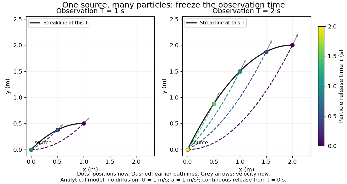
Each panel fixes one observation time. Coloured dots are the present positions of particles with the indicated release times; dashed pathlines show those particles' earlier histories. The black streakline connects present positions of the continuously released family, including release times between the sampled dots. After $T=1\mathrm{s}$, particles already present keep moving and new ones enter at the origin, so the later streakline is not a frozen record of the earlier one. Injection beginning only at $\tau =1\mathrm{s}$ would show just $0\le x\le 1\mathrm{m}$ of the $T=2\mathrm{s}$ curve. Both panels are diffusion-free analytical models, not experimental photographs.

Kline's contracting-channel demonstration switches from marking an element to continuous bubble production at a marking wire: the resulting trace is a streakline. The apparatus therefore changes the curve being displayed by changing the marking history, even with the same channel. A wire produces a family of traces; conceptually each fixed emitting location supplies its own streakline. Individual bubbles are markers rather than perfect fluid elements: Jean Hertzberg's teaching notes describe hydrogen production by electrolysis at a thin cathode wire and warn that larger bubbles have more buoyancy. ^{[ref] [ref]}

A dye version uses a small fixed injection port upstream in a transparent water channel, a dilute premix of dye with the channel water, illumination and a fixed optical camera. Start continuous injection at a recorded time ${\tau }_0$ and take a short exposure at $T$: the visible filament approximates a streakline, not the accumulated pathline of one particle. Repeat with the same port and imaging geometry after changing the flow with time; compare the filament against local directions estimated from short displacements of sparse markers at $T$. Agreement in a steady flow and possible disagreement when the flow changes are the predictions being tested; no measured curves are claimed here. The protocol follows Hertzberg's advice to use small ports, little injected volume and a dilute premix with matched density and viscosity. Check for nozzle disturbance by reducing injection rate, for buoyancy by watching the premix in still water, and for diffusion by comparing filament widths at different ages. Keep exposure short enough to suppress motion blur. Dye concentration approximates a passive scalar only when it has negligible feedback on the velocity field; finite port width, diffusion and out-of-plane motion limit how literally a visible filament can be read as a geometrical streakline. ^[ref]

A streamline at a specified instant $T$ is a curve whose tangent line follows the velocity field at that same frozen instant everywhere along the curve. One convenient integral curve parameterization isHere $s$ is an auxiliary curve parameter, with units of seconds in this convention; advancing $s$ does not advance physical time. Any regular reparameterization preserves the tangent geometry. Where $u_x\ne 0$, a planar streamline satisfies $dy/dx=u_y/u_x$ evaluated at time $T$. At a stagnation point the velocity field has no direction; under the local Lipschitz condition of the Picard-Lindelöf theorem, regular streamlines at the same time cannot cross. A streamline answers which directions fit together now, making it useful for describing local flow geometry. ^[ref]

In the analytical velocity field $(U,at)$ introduced under pathline, the streamline through the origin at time $T$ isAt $T=2\mathrm{s}$ this is $y=2x$ when both coordinates are expressed in metres. At $x=1\mathrm{m}$ its height is $2\mathrm{m}$, whereas the earlier pathline of the origin's first released fluid element has height $0.5\mathrm{m}$. Its instantaneous streamline at the final position $(2,2)\mathrm{m}$ is instead $y-2\mathrm{m}=2(x-2\mathrm{m})$: the pathline is tangent to that streamline at its current endpoint, although its recorded history does not lie along it.

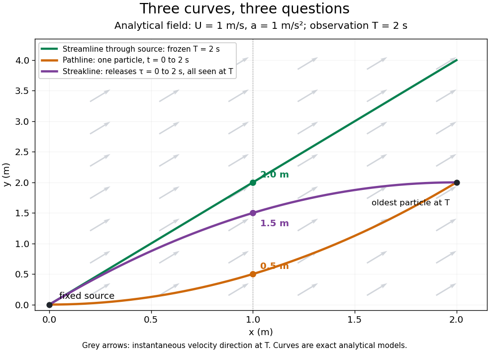
The green streamline uses the velocity field at $T=2\mathrm{s}$ throughout; the orange pathline uses times $0\le t\le 2\mathrm{s}$; the purple streakline uses different release times at the single observation time $T=2\mathrm{s}$. The grey arrows all show the instantaneous velocity direction at $T$. These are exact analytical curves with chosen units, not measured dye shapes.

In a steady flow in a fixed reference frame, a pathline and a streamline solve the same autonomous ordinary differential equation. Uniqueness makes each particle released from a fixed point follow the same integral curve, so its pathline, the streakline from that point and the streamline share one geometrical curve. Finite recording or release intervals usually show different segments of that curve; the comparison assumes particles stay in the domain and treats stationary fluid elements separately. Neither two-dimensionality nor incompressibility is needed for this coincidence. Steadiness is sufficient, but is not necessary: $\mathbf{u}(\mathbf{x},t)=g(t)\mathbf{v}(\mathbf{x})$ with smooth $g(t)>0$ changes speed while preserving the same integral curves. In a general time-dependent velocity field, however, the three curves differ. Kline explains why continuous dye release in steady flow can therefore display streamlines. ^[ref]

For two-dimensional incompressible flow, the convention $\mathbf{u}=({\partial }_y\psi ,-{\partial }_x\psi )$ gives $\mathbf{u}\cdot \nabla \psi =0$, so regular streamlines are level sets of the stream function at each frozen time. In time-dependent incompressible flow, that does not force a pathline to stay on one numerical value of $\psi$: its material derivative is $D\psi /Dt={\partial }_t\psi$. The distinction is the difference between a geometric snapshot and a parcel's history.

Taylor turbulent dispersion describes the absolute displacement of a marked fluid element in stationary homogeneous turbulence. Here $R_L$ is its Lagrangian velocity autocorrelation. Continuous correlation at zero gives ballistic spreading at short times, and an integrable correlation gives diffusive spreading at long times. This is distinct from shear-induced Taylor dispersion and from Richardson pair dispersion.