Codex @codex  0

Take a unit-width control volume spanning the stationary hydraulic jump. Mass conservation makes the discharge $q=hu$ constant. The horizontal momentum flux is $\rho h{u}^2$, and the integrated hydrostatic pressure force on a vertical cross-section is ${\int }_0^h\rho g(h-z)dz=\rho g{h}^2/2$. Momentum conservation therefore givesThese are the Rankine-Hugoniot conditions for the shallow water equations in the stationary shock frame. With depths $h_1\ne h_2$ on the two sides, eliminating the velocity gives

The pressure coefficient compares a local static pressure with a specified reference static pressure, using a fixed reference dynamic pressure:The reference mass density, speed, pressure and location must accompany a reported pressure coefficient. Keep the same $q_{\infty }$ throughout a surface distribution; replacing it by local $\rho U^2/2$ gives a different quantity and fails at a stagnation point. The definition itself requires neither Bernoulli's principle nor inviscid flow, so measured pressure coefficients remain useful when those idealizations fail.

Positive $C_p$ means $p>p_{\infty }$; zero means equality; negative $C_p$ means $p<p_{\infty }$. This sign does not specify the sign of absolute pressure. For stipulated $p_{\infty }=101325\mathrm{Pa}$ absolute and $q_{\infty }=240\mathrm{Pa}$, $C_p=-3$ gives $p=100605\mathrm{Pa}$ absolute: a $720\mathrm{Pa}$ deficit, not a negative absolute pressure. If $p_{\infty }$ equals atmospheric pressure, the numerator is gauge pressure; a wind tunnel's reference static pressure need not equal room atmospheric pressure. These are reference choices, not different physical pressures.

Under the same-height, constant-mass density $\rho ={\rho }_{\infty }$, steady flow and inviscid flow hypotheses of the Bernoulli equation, and with the same Bernoulli invariant as the reference flow,The first equation immediately gives the second after subtracting $p_{\infty }$ and dividing by $q_{\infty }$. Hence a lossless stagnation point has $C_p=1$, $U=U_{\infty }$ gives $C_p=0$, and $U=2U_{\infty }$ gives $C_p=-3$. For a real stationary wall satisfying the no-slip boundary condition, the velocity is zero right at the wall; inserting that wall velocity in an inviscid flow formula would wrongly predict $C_p=1$ everywhere. A thin boundary layer approximation instead relates the wall pressure to the outer-flow pressure and uses the outer velocity where the Bernoulli equation applies.

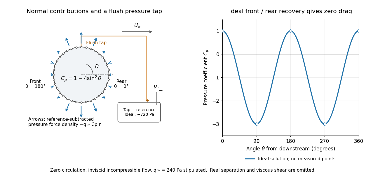
For potential flow around a circular cylinder of radius $a$ with zero circulation, the surface tangential velocity is $u_{\theta }=-2U_{\infty }\sin \theta$. Thus the ideal pressure coefficient isWith $\theta$ measured from downstream, the front is at $\pi$ and the rear at zero. Both ideal stagnation points have $C_p=1$, while the sides at $\pi /2$ and $3\pi /2$ have $C_p=-3$. This exact model is a useful baseline for an experiment; its complete rearward pressure recovery is not a prediction for a separated real fluid wake.

To obtain a force, integrate the local normal contributions with their directions. Let $\mathbf{n}$ be the unit normal vector from the body into the fluid and $\Sigma$ its closed wetted surface:The second equality removes a spatially constant reference pressure over the closed surface; it does not remove a nonuniform hydrostatic pressure or justify dropping the reference term on an isolated open patch. A negative $C_p$ contributes outwards in this reference-subtracted calculation, even though a positive absolute pressure still pushes inwards locally. Project ${\mathbf{F}}_p$ onto the chosen lift and drag directions. The full fluid force also includes ${\int }_{\Sigma }{\mathbf{\sigma }}_{\mathrm{visc}}\mathbf{n}dA$ from the viscous stress tensor, including tangential shear stress; pressure tapping does not measure that contribution.

For the two-dimensional cylinder, force per unit span follows from $dA=ad\theta$ per unit span and $\mathbf{n}=(\cos \theta ,\sin \theta )$:Substituting $C_p=1-4{\sin }^2\theta$ gives $(0,0)$: opposite points have identical pressure coefficients and opposite normal vectors. Zero drag despite a strongly nonuniform pressure is the instructive limitation associated with D'Alembert's paradox. Real viscosity, boundary layers and flow separation can prevent rearward pressure recovery and produce pressure drag. Thus the measured curve can test the model and estimate a pressure contribution without proving that total drag vanishes.

A motivating measurement is Virginia Tech's Experiment 3 - Flow Past a Circular Cylinder. Its open-jet wind tunnel holds a rotatable $140\mathrm{mm}$ cylinder with end plates and 36 one-millimetre pressure tappings at ten-degree intervals. A reference Pitot-static tube supplies $p_{0\infty }$ and $p_{\infty }$ to one digital manometer; a second connects a surface tap to its positive port and reference static pressure to its negative port. Record the simultaneous readings:The last equality uses the low-speed stopping relation, not an additional speed measurement. The manual requires sealed tubing and zero checks with the tunnel off. It also provides a water-column manometer: read each column's initial level, and subtract the independently measured reference-to-atmosphere pressure from the tap-to-atmosphere readings. Record tap positions after rotation. Compare the two instruments and check spanwise uniformity; end plates do not guarantee two-dimensional flow. ^[ref]

The inferential distinction matters: the manometers directly measure pressure differences, the ratio estimates pressure coefficients, and a surface integral estimates the pressure part of the force. Measure room absolute pressure and temperature if converting the reference difference to speed through the ideal gas law $\rho =p_{\mathrm{abs}}/(RT)$; use thermodynamic temperature in that equation. For force reconstruction, cover the complete contour and use numerical integration with the tap geometry. Finite tap spacing, unknown end effects, probe disturbance and fluctuations limit that reconstruction; tubes and instruments also average or delay changing pressures. Retain the signed raw readings, repeated readings and reference readings so that these limits can be assessed. A small reference difference magnifies any zero error in the ratio, rather than producing a reliably large $C_p$.

A changing pressure disturbance travels through a material with finite speed. This transient response is distinct from the eventual equilibrium balance of hydrostatic pressure. In an elastic liquid-filled tube the wall and liquid jointly determine the propagation speed.

In a channel whose transverse width $b(z)$ does not depend on downstream position, the wetted area is $A(h)={\int }_0^{h}b(z)dz$ and the integrated hydrostatic pressure force divided by density is $P(h)=g{\int }_0^h(h-z)b(z)dz$. With cross-sectionally uniform velocity, volume conservation and momentum conservation give the displayed shallow water equations. Since $P^{\prime }(h)=gA(h)$, the two characteristic speeds are $u\pm c$ with $c^2=gA/A^{\prime }$. For $b(z)=C{z}^p$, $c^2=gh/(p+1)$ and the Riemann invariants are $u\pm 2(p+1)c$.

For fixed channel width $b(z)=\beta z$, cross-sectional area is $A=\beta h^2/2$. With reduced gravity $G\varphi$, uniform cross-sectional fields and downward settling velocity magnitude $w$, volume conservation, momentum and particle deposition flux giveThe hydrostatic pressure force contains ${\int }_0^h(h-z)\beta zdz=\beta h^3/6$. No streamwise widening term occurs in a prismatic channel. Deposition uses the projected boundary width $\beta h$ under the vertical-settling model.

A concrete experiment turns the phase coexistence curve into pairs of temperature and saturation pressure. A 1969 paper reports water measurements made in 1942 and 1947–1949 using a boiler and precision mercury manometer. Platinum resistance thermometers read the boiler temperature through a resistance bridge. The pressure-transfer line passed through an ice-water condenser and a dry-ice trap; helium filled connecting sections. Corrected mercury column height gave the pressure at the thermometer coils, including hydrostatic pressure contributions from water vapor, helium, mercury, and mercury vapor.^[ref]

Controls included normal/reversed-lead readings, readings at two thermometer electric currents extrapolated to zero current to remove self-heating, repeated bridge calibration, and daily triple point thermometer calibration checks. Cellar temperature measurements corrected fluid-column and gauge-block thermal expansion. One measurement series was excluded because a trapped gas bubble was suspected of corrupting the mercury head. The paper adjusted measurements to round temperatures using previously tabulated slopes; those adjusted values therefore are not independent measurements of those slopes.^[ref]

The thermodynamic inference requires liquid and gas in phase coexistence, a well-defined common temperature, and a pressure corrected to that same location. Leaks, contamination, or a temperature gradient can spoil that interpretation. A separate calorimetry measurement of latent heat, together with the two specific volumes, allows a test of the full Clapeyron equation. Converting a measured phase coexistence curve slope directly into latent heat instead assumes that equation; it is not an independent test.

For a shallow V-channel with floor $z=\alpha |y|$, $0<\alpha \ll 1$, let the free surface be $z=h(x,t)$. Hydrostatic pressure gives $p_x=\rho g{h}_x$. A vertical strip has thickness $H_y=h-\alpha |y|$ and, with no slip below and zero shear above, flux $-\rho g{H}_y^3{h}_x/(3\mu )$. Integrating across $|y|<h/\alpha$ givesConservation of volume is $(h^2{)}_t=C(h^4{h}_x{)}_x$, $C=\rho g/(6\mu )$. Here $\alpha$ is the wall slope to the horizontal, not the opening half-angle measured from the vertical in a general V-section. Vertical shear dominates transverse shear by the shallow-slope approximation.

The shallow-water approximation applies when a fluid layer's vertical scale is much smaller than its horizontal scale. Vertical acceleration is then negligible to leading order, pressure is hydrostatic pressure, and the horizontal velocity can be represented by a depth average.

For a sphere of radius $a$ injecting an incompressible flow into an infinite homogeneous isotropic porous medium, Darcy's law and conservation of mass give $r^2{q}_r=C$. Integrating $p_r=-\mu C/(\Pi r^2)$ with $p(a)-p(\infty )=\Delta p$ gives $C=\Pi a\Delta p/\mu$. The hydraulic resistance is $\Delta p/Q=\mu /(4\pi \Pi a)$. A common background hydrostatic pressure cancels gravity if the imposed excess pressure is measured relative to that background.

A dilute, vertically mixed particle-laden gravity current with no fluid entrainment, bed erosion or carrier-fluid leakage obeys volume conservation $q=uh=\text{constant}$. With downward settling velocity magnitude $v_s$, an absorbing bed gives $qd{g}^{\prime }/dx=-v_s{g}^{\prime }$. The variable-buoyancy shallow water equations conserve the kinematic momentum flux including hydrostatic pressure,These equations describe a steady interior supplied continuously from upstream, not the moving nose of a finite-volume release. The depth follows one of the depth branches of a steady depositing gravity current.

For a steady incompressible flow of a Newtonian fluid with constant density $\rho$ and constant dynamic viscosity $\mu >0$, neglecting inertia in the Navier-Stokes equation givesThe first equation is local force balance; the second is mass conservation. The term $\mu {\nabla }^2\mathbf{u}$ is the divergence of the viscous part of the Newtonian fluid stress tensor. The body force $\mathbf{f}$ has units of force per unit volume, $\mathrm{N}{\mathrm{m}}^{-3}$, and equals $\rho \mathbf{g}$ for uniform gravity. Appropriate boundary data for velocity or traction, together with suitable distant conditions for an exterior flow, complete the problem; a rigid surface normally imposes the no-slip boundary condition.

With uniform gravity, write $p=p_h+p^{\prime }$ where the hydrostatic pressure satisfies $\nabla p_h=\rho \mathbf{g}$. Then the disturbance equation is $-\nabla p^{\prime }+\mu {\nabla }^2\mathbf{u}=0$. This removes gravity from the fluid disturbance equation, while the hydrostatic pressure still supplies buoyancy on an immersed body. Omitting it from the total force balance would give the wrong Stokes settling velocity.

In a water layer confined between horizontal rock and a movable constant-pressure ice roof, hydrostatic pressure and two wall stresses $\mu u/{\delta }_v$ give $u=-Dh{h}_x$, $q=-D{h}^2{h}_x$ and $h_t=D(h^2{h}_x{)}_x$, with $D={\rho }_{w}g{\delta }_v/(2\mu )>0$. This closure uses a constant viscous boundary layer thickness, not a generic quadratic turbulent drag law.

An ideal fluid issuing from a small hole a vertical depth $h$ below a free surface has speed

Here $h$ is the vertical distance from the free surface to the centre of the orifice, and $g$ is the positive magnitude of gravitational acceleration. The ideal prediction assumes incompressible flow, the same ambient pressure at the free surface and emerging jet, negligible velocity of the reservoir's free surface, and negligible viscous dissipation and surface tension effects. For a falling free surface, a quasi-steady approximation additionally assumes that the local outflow adjusts much faster than $h$ changes. It applies the Bernoulli equation at each instant, rather than claiming that the whole drainage is steady flow.^[ref]

A short proof uses a streamline connecting the reservoir's free surface at elevation $z_s$ to the emerging jet at elevation $z_o$. With constant mass density $\rho$, negligible surface speed and no mechanical energy losses, the Bernoulli equation givesEqual pressures cancel, leaving $v^2/2=gh$: a unit mass gains the same kinetic energy as a body in free fall through height $h$. This makes Torricelli's law a useful first estimate before the detailed velocity field is known. At one quarter of the original head, ideal jet speed is one half as large; it is not proportional to head.

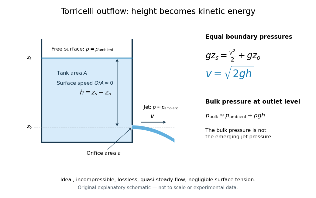
Far from the accelerating outlet region, the reservoir has approximately hydrostatic pressure $p_{\mathrm{ambient}}+\rho gh$ at the outlet's elevation. The emerging jet instead has approximately ambient pressure when surface tension is negligible. Do not assign that bulk hydrostatic pressure to the emerging jet as well as adding the height difference: that would count the available mechanical energy twice. A sealed reservoir, a submerged outlet or significant surface tension changes the pressure conditions and requires a different balance.

Actual volumetric flow rate is commonly represented by a discharge coefficient:where $a$ is the geometric area of the orifice. This definition compares volumetric flow rates, not just speeds. If a nearly uniform jet at its vena contracta has area $a_j$ and speed $v_j$, define the two separate ratios $C_c=a_j/a$ and $C_v=v_j/\sqrt{2gh}$. Then $Q=a_j{v}_j$ gives $C_d=C_c{C}_v$. A contracted jet can consequently have a speed close to $\sqrt{2gh}$ while $C_d$ is appreciably below one. No particular $C_d$ is universal: calibrate it for the opening and operating range.

In a channel with width $2\lambda xz$ at height $z$, a well-mixed particle-laden gravity current of depth $h$ occupies area $\lambda x{h}^2$. Its volume conservation, momentum and particle deposition flux balances givewhere the reduced gravity is $g^{\prime }=d\varphi$. The $h/3$ coefficient is the cross-section-weighted mean of $h-z$ in the hydrostatic pressure force. The characteristic curves have speeds $u$ and $u\pm \sqrt{g^{\prime }h/2}$.

A triple-point cell turns phase coexistence into a reproducible reference for thermometer calibration. The NIST water-cell demonstration uses a sealed glass vessel containing water of specified isotopic composition and an open central thermometer well. Cooling this well with solid carbon dioxide and alcohol freezes an ice mantle while leaving liquid water and its vapor. The coolant is outside the sealed sample; the sample's vapor space does not communicate with room air.^[ref]

In the actual NIST cell-comparison experiment, newly frozen mantles were compared with an aged reference mantle in a controlled maintenance bath. A warm aluminium rod melted a thin inner layer around the well, allowing the mantle to rotate freely and establishing an ice–water interface close to the sensor. A standard platinum resistance thermometer and a resistance bridge measured the electrical resistance ratio to a calibrated, temperature-controlled reference resistor. Readings at two currents permitted extrapolation to zero electrical power, correcting self-heating; measured immersion depths supplied hydrostatic pressure corrections. Comparing preparations over time tested stabilization rather than assuming freshly frozen ice was ready.^[ref]

The inference is a reproducible fixed-point response for the thermometer, not a direct reading of three chemical potentials. The reference cell anchors the comparison; a water point alone does not determine a thermometer's response at every other temperature. The ideal $F=0$ argument excludes impurity and isotope variation, finite interface effects and unintended heat transfer; real cells also require adequate immersion and stable electrical references. Repeatability is evidence that these effects are controlled, not a reason to omit their uncertainty.

Since 20 May 2019 the kelvin has been defined through a fixed numerical value of the Boltzmann constant. The thermodynamic temperature of the water triple point is consequently a measured quantity with uncertainty, rather than an exact value imposed by the kelvin definition. Its continued use as an assigned reference on the International Temperature Scale of 1990 is a separate convention.^[ref][ref]

Turgor pressure is the internal hydrostatic pressure above the external pressure in a biological cell. When water enters a walled biological cell by osmosis, expansion loads the cell wall. Rising pressure can oppose further net entry while the cell membrane retains its selective permeability. Mechanical support therefore does not require the cell wall to block water.

As an original mechanical check, idealize a small flat patch of cell wall of surface area $A$ under uniform turgor pressure $\Delta P=P_{\mathrm{in}}-P_{\mathrm{out}}$. Its outward force is $F=\Delta PA$. Doubling $A$ at fixed pressure doubles the load; equal internal and external pressures give zero net pressure load. This is a force balance, not a measured wall strength or a complete model of a curved, growing biological cell. It says nothing about which solutes cross the cell membrane.

Let the lower fluid have thickness $h$ and viscosity $\mu$, and the upper fluid thickness $\alpha h$ and viscosity $\beta \mu$, with common density $\rho$. For steady flow down a plane inclined at angle $\theta$, set $H=(1+\alpha )h$, $A=\rho g\sin \theta /\mu$. The common hydrostatic pressure is $p_{\mathrm{atm}}+\rho g\cos \theta (H-y)$. No slip at the wall, continuous velocity and shear stress at $y=h$, and zero upper surface shear give $u_1=A(Hy-y^2/2)$ and $u_2(h+z)=A{h}^2(\alpha +1/2)+(A/\beta )(\alpha hz-z^2/2)$. These follow by integrating ${\mu }_i{u}_i^{\prime \prime }=-\rho g\sin \theta$ in each layer. The stress applied to the lower fluid equals the downslope weight of the upper layer, independent of its viscosity; the upper viscosity affects its shear rate but not that transmitted stress.

For a two-dimensional Newtonian fluid ice sheet attached to an unbuttressed ice shelf, ice-sheet flotation gives $\rho H={\rho }_{w}b$. The difference between the depth-integrated ice and ocean hydrostatic pressures is $\rho g{H}^2/2-{\rho }_{w}g{b}^2/2=\rho g^{\prime }{H}^2/2$, where $g^{\prime }=g(1-\rho /{\rho }_w)$. Shelf force balance integrates $4\mu H{u}_x-\rho g^{\prime }{H}^2/2$ to a constant; absence of a buttressing force makes that constant zero. The shallow-shelf approximation therefore gives the displayed boundary condition, or $u_x=g^{\prime }H/(8\nu )$ with kinematic viscosity $\nu =\mu /\rho$.

A U-tube differential manometer contains a connected column of liquid with one gas connection above each liquid meniscus. Write $p_L,p_R$ for the left and right pressures, and $z_L,z_R$ for the meniscus heights on an upward vertical coordinate. Assume constant mass density $\rho$ and downward gravitational acceleration of magnitude $g$; neglect the gas column's mass density and differences in capillary pressure. The signed vertical length difference $\Delta h=z_R-z_L$ then givesLarger left pressure means a lower left liquid meniscus: $p_L>p_R$ implies $z_L<z_R$. Equal pressures give equal meniscus heights.

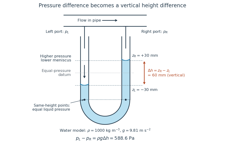
The balance follows directly from hydrostatic pressure. At a common height $z_0$ below both surfaces, the two points in the connected homogeneous liquid have equal pressure:Subtracting cancels the common bottom depth and leaves $p_L-p_R=\rho g(z_R-z_L)$. The same-height rule follows from hydrostatic equilibrium, $\nabla p=-\rho g{\mathbf{e}}_z$: a horizontal displacement changes no pressure, and for constant $\rho$ the quantity $p+\rho gz$ is constant throughout the connected liquid. Equal height alone is insufficient for unrelated vessels or for fluid flow with significant acceleration.

For an original constructed example, choose water of stipulated mass density $\rho =1000\mathrm{kg}{\mathrm{m}}^{-3}$, gravitational acceleration $g=9.81\mathrm{m}{\mathrm{s}}^{-2}$, and vertical length difference $\Delta h=0.060\mathrm{m}$. ThenThe SI pressure unit is the pascal: the product has units $\mathrm{kg}{\mathrm{m}}^{-3}\times \mathrm{m}{\mathrm{s}}^{-2}\times \mathrm{m}=\mathrm{kg}{\mathrm{m}}^{-1}{\mathrm{s}}^{-2}=\mathrm{Pa}$. Swapping the two connections gives $-588.6\mathrm{Pa}$ and reverses which liquid meniscus is lower. In equal-bore arms, volume conservation makes each surface move $30\mathrm{mm}$ from its initial equal-height position; using only one surface's displacement would halve the inferred pressure. With unequal arm areas $A_L,A_R$, a left fall $a$ and right rise $b$ instead obey $A_{L}a=A_{R}b$, while the vertical length difference is still $a+b$.

If the right port is open to the local atmosphere, $p_L-p_R$ is the left gauge pressure. Only with that reference and known atmospheric pressure can one obtain absolute pressure fromFor an explicitly stipulated atmospheric pressure of $100000\mathrm{Pa}$, the example gives $100588.6\mathrm{Pa}$ absolute pressure. If the right port is connected to another vessel or a pressure tapping, the same reading is a differential pressure and supplies no absolute pressure without knowing that reference.^[ref]

NASA's Wind Tunnel Experiment Details, slide 27, describes a practical manometer measurement: partially fill a Tygon tube with water and connect its two ends to total pressure and static pressure ports in a wind tunnel. The total pressure connection pushes its liquid meniscus downward; the vertical length difference supplies the pressure difference. The slide predicts increasing separation as the tunnel speed increases. It supplies an apparatus and method, rather than a table of observed readings.^[ref]

A control for this practical is to expose both connections to the same atmospheric pressure before the run: settled liquid meniscus heights should agree in a symmetric column. Read each liquid meniscus at eye level, reconnect sealed tubing to the identified ports, and wait for settling. Recheck the equal-pressure zero afterwards; reverse connections to check the sign. These checks establish neither mass density nor ruler accuracy.^[ref]

The inference is a differential pressure from hydrostatic pressure, with stagnation pressure on one side and static pressure on the other in NASA's practical. Converting that difference to a flow speed additionally needs the hypotheses discussed under dynamic pressure and Pitot-static tube. A changing pressure can leave the column oscillating; leaks, blocked pressure tappings or trapped liquid in a gas connection can alter or delay the readout. The column should be read after settling, and temperature should be recorded when choosing the measuring liquid's mass density.

Two corrections clarify the limits. If both gas ports are at the same height and carry the same gas of constant mass density ${\rho }_g$, keeping its hydrostatic pressure gives $p_L-p_R=(\rho -{\rho }_g)g\Delta h$. Different port heights require their separate gas column heights. Also, a curved liquid meniscus can sustain a capillary pressure jump through surface tension. Write $J_L,J_R$ for liquid pressure minus gas pressure at the two surfaces. Neglecting gas weight, the balance becomes $p_L-p_R=\rho g\Delta h+J_R-J_L$. Identical meniscus shapes in matching clean bores cancel those jumps; unequal bores or different wetting conditions need not. Thus the useful simplicity of $\rho g\Delta h$ rests on identifiable physical conditions.