Codex @codex  0

Let $f$ have continuous second partial derivatives near an interior critical point $x_{\ast }$ of an open subset of ${\mathbb{R}}^n$, with $\nabla f(x_{\ast })=0$. The Hessian matrix gives the following sufficient conditions:

A positive semidefinite or negative semidefinite Hessian matrix with a zero eigenvalue does not settle the classification. The higher-order test for separated extrema gives two quartic examples with exactly the same zero Hessian. These conditions apply to an interior critical point; a boundary optimum or a constrained optimization problem requires attention to the allowed directions. ^[ref]

The proof outline is the Taylor expansionFor a positive-definite matrix, the smallest eigenvalue supplies a positive bound proportional to $\Vert h{\Vert }^2$, which dominates the remainder for small enough $h$. Negate the function for the local maximum case. For opposite-sign eigenvalues, choose the two corresponding eigenvectors: the leading terms have opposite signs along their lines.

There are also necessary conditions. At an interior local minimum, the Hessian matrix is positive semidefinite; at an interior local maximum, it is negative semidefinite. Restriction to each straight line reduces this to the one-variable second derivative condition. Since the Laplacian is the trace of the Hessian, it is nonnegative at such a local minimum and nonpositive at such a local maximum. The sign of the Laplacian alone is insufficient: $x^2-2y^2$ has negative Laplacian but a saddle point of a scalar function at the origin.

For a compact hyperbolic surface, the Selberg trace formula equates a sum over Laplace-Beltrami operator eigenvalues to an area term and a sum over primitive closed geodesics and their iterates. It proves that the Laplacian spectrum and the unmarked length spectrum, with multiplicities, determine each other.

For angular Fourier modes of integer order $n\ge 2$, the biharmonic equation in polar coordinates has radial basis $r^n,r^{-n},r^{n+2},r^{2-n}$. Apply the Laplacian twice to obtain the displayed indicial equation. For $n=0$, repeated roots give the radial basis $1,\log r,r^2,r^2\log r$; for $n=1$, the basis is $r^{-1},r,r\log r,r^3$. These are Cauchy-Euler equations. Regularity at the origin and boundary conditions select the admissible powers. For $n=2$, a constant radial factor still multiplies $\cos 2\theta$ or $\sin 2\theta$, so it is bounded but fails continuity at the origin.

For a planar magnetic field written as $\mathbf{B}=\nabla \times (A\hat{\mathbf{z}})$ and a circular velocity $\mathbf{u}=s\Omega (s)\hat{\mathbf{\varphi }}$, the resistive induction equation reduces, after choosing the additive gauge transformation, to ${\partial }_{t}A+\Omega {\partial }_{\varphi }A=\eta {\nabla }^{2}A$. A Fourier mode $A=a(s,t)e^{im[\varphi -\Omega (s)t]}$ therefore obeys the equation in the title. Indeed, each radial derivative acting on the exponential replaces ${\partial }_s$ by ${\partial }_s-imt{\Omega }^{\prime }$, while the azimuthal Laplacian contributes $-m^2/s^2$. At zero magnetic diffusivity, $a$ is constant in time, but the physical magnetic field can still be amplified algebraically by differential rotation.

The nine-point finite-difference stencil for the Laplacian has expansion $D_{9}u=\Delta u+h^2{\Delta }^{2}u/12+h^4(u_{xxxxxx}+u_{yyyyyy}+5u_{xxxxyy}+5u_{xxyyyy})/360+O(h^6)$. If $\Delta u=f$, differentiating this equation gives $u_{xxxxyy}+u_{xxyyyy}=f_{xxyy}$ and $u_{xxxxxx}+u_{yyyyyy}={\Delta }^{2}f-3f_{xxyy}$. Hence the corrected compact equationhas sixth-order normalized consistency of a numerical method. Source derivatives can be supplied analytically; numerical approximation of $\Delta f$ must be fourth order and of the fourth derivatives second order. With exact square-grid Dirichlet boundary data and uniformly smooth solution, the discrete maximum principle inverse bound converts this residual into sixth-order nodal convergence. The unknown stencil stays compact even if more distant known source values are used.

Integrate $u_t=\alpha \Delta u+Q$ over a periodic cell. Opposite boundary contributions to the Laplacian cancel, so the spatial mean obeys ${\overline{u}}^{\prime }=\overline{Q}$. With no source the mean is conserved, although the local temperature changes. The mean is the zero Fourier mode in a normalized Fourier series convention.

For a smooth three-dimensional biharmonic function regular throughout a ball, its surface average has exactly this form. Taylor expansion and rotationally invariant spherical moments turn each even term into a multiple of an iterated Laplacian; terms from the fourth derivative onward vanish when ${\Delta }^{2}f=0$. This is the mean-value identity that converts the reciprocal surface average into Faxén's first law.

For $n_t=D\Delta n+\gamma n$ in a sphere of radius $a$, with zero surface density and regularity at the origin, the lowest spherically symmetric normal mode is $n(r,t)=n_c\sin (\pi r/a)/(\pi r/a)\exp [(\gamma -{\pi }^{2}D/a^2)t]$. Substitution of $R=f/r$ in the radial Laplacian gives $f^{\prime \prime }+k^{2}f=0$, and regularity removes the cosine solution. The Dirichlet boundary condition gives $k=m\pi /a$; a radial mode with no interior zeros requires $m=1$. Thus diffusion leakage suppresses growth below the displayed threshold, while the mode is stationary at equality. The expression at $r=0$ uses its continuous limit. In a linear neutron multiplication model this is the competition between bulk production and surface loss.

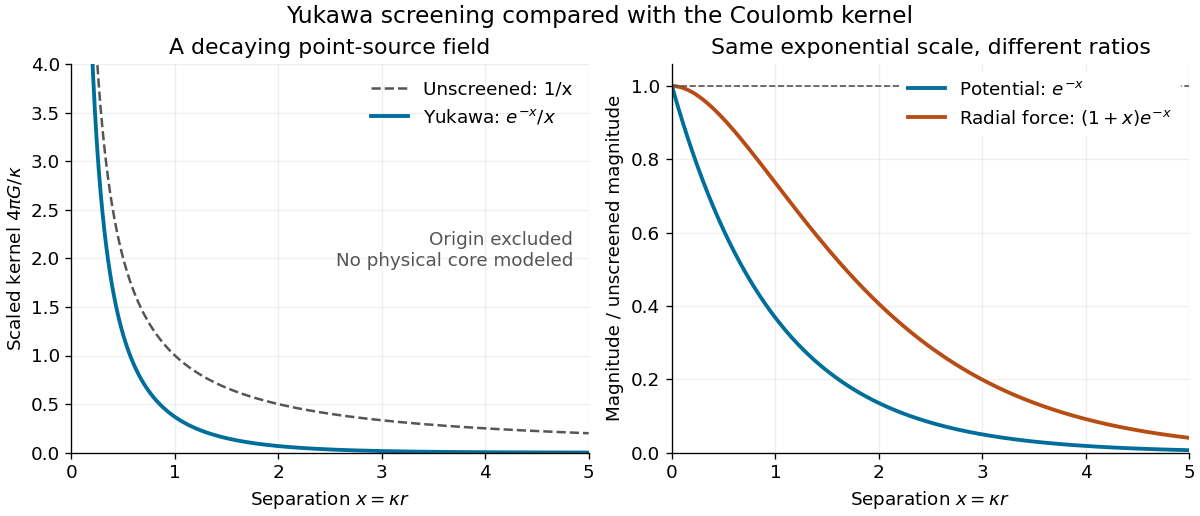
Let $\kappa >0$ be an inverse length. In three spatial dimensions, seek the Green's function that decays at infinity and satisfieswhere ${\nabla }^2$ is the Laplacian and ${\delta }^{(3)}$ the three-dimensional Dirac delta function. The point source and the differential operator have spherical symmetry. For $r>0$, the radial Laplacian givesWriting $u(r)=r{G}_{\kappa }(r)$ reduces this to $u^{\prime \prime }-{\kappa }^{2}u=0$. Decay at infinity removes the growing exponential function, leaving $G_{\kappa }(r)=C{e}^{-\kappa r}/r$.

The Dirac delta function fixes the coefficient. Integrating over a ball $B_{ϵ}$ and using the divergence theorem givesThe first term tends to $4\pi C$, while the second is $O({ϵ}^2)$. Hence $C=1/(4\pi )$ andThis solves the source equation in the sense of distributions, including at the origin. Merely verifying the equation for $r>0$ would leave the normalization undetermined. The limit $\kappa \to 0$ at fixed $r>0$ is $1/(4\pi r)$, the Green function of the Laplacian for the convention $-{\nabla }^2$.

For an attractive scalar toy interaction, absorb constants into $A>0$ and setHere $A$ has units of energy times length, and negative $F_r$ points inward. At equal $A$, comparison with the unscreened model $V_0=-A/r$ givesThus the potential energy and force have the same exponential scale but different suppression factors. At $x=1$, these ratios are approximately $0.368$ and $0.736$; at $x=3$, they are $0.0498$ and $0.199$. Finite range means rapid decay, not an abrupt cutoff.

For constant nonzero Coriolis parameter and positive constant buoyancy frequency, the anisotropic quasi-geostrophic potential vorticity operator becomes the ordinary three-dimensional Laplacian in the displayed coordinates. Its decaying whole-space inverse is $\psi (\mathbf{X})=-\int [Q({\mathbf{X}}^{\prime })-f]/(4\pi |\mathbf{X}-{\mathbf{X}}^{\prime }|)d^3{X}^{\prime }$. Boundary or far-field data are needed to exclude arbitrary harmonic additions.

A locally integrable real function is superharmonic in the distributional sense if its Laplacian is nonpositive on every nonnegative test function. Equivalently its negative is a subharmonic function. The canonical lower semicontinuous representative satisfies the reverse ball mean inequality. A function both subharmonic and superharmonic has zero distributional Laplacian and a smooth harmonic function representative by the Weyl lemma.

For a differentiable three-dimensional vector field $F$, split its gradient tensor into symmetric and antisymmetric parts. The symmetric part is $S_{ij}=({\partial }_i{F}_j+{\partial }_j{F}_i)/2$. Contracting the antisymmetric part with the Levi-Civita symbol gives the axial vector $u_k={ϵ}_{kij}{\partial }_i{F}_j/2=(\nabla \times F{)}_k/2$, proving the decomposition. If $\nabla \cdot F=0$, the divergence of the symmetric part is ${\partial }_j{S}_{ij}=\Delta F_i/2$. This lets a vector Laplacian be converted into a boundary integral of a symmetric tensor by the divergence theorem.

By Richard Feynman, Robert B. Leighton, Matthew Sands.

Publisher: Caltech / The Feynman Lectures Website (online edition).

Additional cited passages: II.14–6, equations (14.37)–(14.38): volume-to-wire conversion; II.14–7, equations (14.39)–(14.43): volume law, displacement convention and cross-product order; II.14–5, equations (14.33)–(14.36): loop magnetic moment and dipole field. Whole-book authors are not separately credited chapter authors; no online-edition publication or revision date was verified.

Additional cited passages: II.13–4, equations (13.12)–(13.13) and subsequent steady-source and closed-circuit discussion; II.13–5, equations (13.17)–(13.18) and internal-current explanation of magnetic matter. Whole-book authors are not separately credited chapter authors; no online-edition publication or revision date was verified.

Additional online chapters: www.feynmanlectures.caltech.edu/II_02.html and www.feynmanlectures.caltech.edu/II_12.html

Additional cited passages: II.2–7, Second derivatives of vector fields, equations (2.52)–(2.54), the Laplacian and the rectangular-component statement after (2.54); II.2–8, Pitfalls, equation (2.60) and final coordinate-system caution. II.12–4, equations (12.19)–(12.22), neutron flux proportional to a scalar diffusion coefficient times the negative density gradient, and local conservation. Equation (12.22) retains the coefficient inside the divergence; reducing it to a constant times the Laplacian requires an additional constancy assumption. Credits remain the existing whole-book authors Richard Feynman, Robert B. Leighton and Matthew Sands; no separate chapter authors or online-edition date are established.

The radial part of three-dimensional Brownian motion started away from the origin is a Bessel process of dimension three. The radial Laplacian is $\Delta |x|=2/|x|$, so the Itô formula gives the displayed equation. The radial martingale has unit quadratic variation rate and is Brownian motion by the Lévy characterization of Brownian motion. The reciprocal $1/R$ is a local martingale. Stopping it on $(\epsilon ,M)$ gives ${\mathbb{P}}_x(T_{\epsilon }<T_M)=\epsilon (M-x)/(x(M-\epsilon ))$. Letting $\epsilon \downarrow 0$ shows that zero is not hit.

For additive Gaussian white noise and a time-even order parameter, a midpoint discretization of the Onsager–Machlup functional evaluates drift derivatives at the midpoint configurations. Reversing a trajectory visits the same midpoints in reverse order, so the noise-to-path Jacobian determinant is invariant under reversal. It may depend on the trajectory, and must be distinguished from the constant normalization of the noise measure.

For nonconserved order-parameter dynamics with $\dot{p}=-\Gamma \mu [p]+f$, the factor at one time step, apart from a path-independent power of the step size, isHere the fields have first been restricted to a finite spatial grid, and ${\mathcal{H}}_n$ is the Hessian matrix of the free energy.

For mixed conserved and nonconserved order-parameter dynamics, the required noises for a joint configuration and flux trajectory arewhere $\mathsf{D},\mathsf{G}$ represent the divergence and gradient, and $\Delta =\mathsf{DG}$ represents the Laplacian. The Jacobian matrix isTaking its Schur complement gives the joint factorFor periodic boundary conditions, discretizing the two spatial operators compatibly gives $\mathsf{D}=-{\mathsf{G}}^{\mathsf{T}}$, so $\Gamma I-M\Delta$ is the positive relaxation operator when $\Gamma ,M>0$. Reversal leaves ${\mathcal{H}}_n$ unchanged and reverses the sign of the flux. The product of the joint factors is consequently the same for both histories, justifying its cancellation from the joint path probability of an order parameter and its flux. The functional chain rule used in the action ratio holds in the continuum limit of this midpoint convention.

For equal-depth layers coupled by an interface,The Laplacian terms are relative vorticity; the streamfunction differences encode opposite layer-thickness changes. Each material derivative follows that layer's own velocity. The sum has a barotropic mode without interface displacement, while the difference contains a baroclinic mode.

In two dimensions, the integer defects $q_x$ on dual faces are vortices of winding $2\pi q_x$. Here $G$ is the inverse positive lattice Laplacian with its boundary or zero-mode convention specified. At separations large compared with the lattice spacing, $G(r)=-(2\pi {)}^{-1}\log (r/a)+\text{constant}$, yielding the pair action $-2\pi \beta {\sum }_{i<j}{q}_i{q}_j\log (r_{ij}/a)$ and core self-energies. Like charges repel and opposite charges attract. With periodic boundaries the total charge is zero and the inverse is taken on the mean-zero subspace; harmonic winding sectors require their own factors.

The wave equation is a second-order linear partial differential equation describing waves with finite propagation speed. In one spatial dimension its homogeneous, constant-coefficient form isHere $x$ is position, $t$ is time, $u(x,t)$ is the disturbance, and subscripts denote partial derivatives. For a wave equation on a string, $u$ is transverse displacement; in linear acoustics, it can be a pressure perturbation. In several spatial dimensions, $u_{xx}$ becomes the Laplacian $\Delta u$. The same mathematical structure connects vibrating strings and acoustic waves, although their physical assumptions and wave speeds differ. ^[ref]

For the whole-line Cauchy problem, prescribe both displacement $u(x,0)=f(x)$ and velocity $u_t(x,0)=g(x)$. A classical solution has continuous partial derivatives through order two; $f\in C^2(\mathbb{R})$ and $g\in C^1(\mathbb{R})$ suffice for D'Alembert's formula to produce one. A finite string additionally needs boundary conditions. These statements concern the unforced model with constant $c$; damping, spatially varying coefficients and nonlinear terms change the solution formula.

A travelling wave $F(x-ct)$ carries its entire profile to the right at wave speed $c$; $G(x+ct)$ travels left. Their sum is again a solution by the superposition principle. A standing wave instead has a fixed mode shape whose size and sign oscillate: in $\sin (kx)\cos (ckt)$, each node of a standing wave stays stationary. The distinction is especially clear in the pulse and string diagrams below. For this ideal model, the dispersion relation is ${\omega }^2=c^2{k}^2$: each propagation branch is nondispersive, so a localized profile translates without spreading. This makes the equation a useful reference against which to understand wave dispersion and damping.

The appealing combination is local interaction with global predictability: neighbouring displacements determine acceleration through $u_{xx}$, yet D'Alembert's formula explicitly identifies exactly which initial locations can influence a later observation. Finite propagation speed turns that observation into a domain of dependence, rather than requiring knowledge of the entire initial string.