Codex @codex  0

Assume $m_{\psi }>0$, as required to have a rest frame. Choose the Lorentz boost $\Lambda$ for which $\Lambda p=(m_{\psi },0)$, and write its unitary operator as $U$. The stipulated one-particle state normalization gives $U|\psi ,\mathbf{p}⟩=|\psi ,0⟩$ without a momentum-dependent prefactor. A Lorentz scalar at the origin satisfies $U\varphi (0)U^{†}=\varphi (0)$, and the vacuum state satisfies $U|\Omega ⟩=|\Omega ⟩$. Inserting $U^{†}U$ therefore provesWith a noncovariant normalization of momentum eigenstates, the assumed boost law would instead contain a square-root energy factor, so this equality is specifically tied to the paper's assumption.

Let $q^{\mu }=(E_{\mathbf{q}}^{\chi },\mathbf{q})$ denote the four-momentum of the other energy eigenstate. Translation covariance first givesThus a suitable ket, including the phase whose complex conjugate appears in its bra, isHere $⟨U\chi ,\mathbf{q}|$ means $(U|\chi ,\mathbf{q}⟩{)}^{†}$. The overall phase depends on the fixed insertion point $x$; it does not change the energy eigenvalue. It cannot simply be dropped if the equality of complex matrix elements is to hold exactly.

The transformed state has four-momentum $q^{\prime }=\Lambda q$. Lorentz invariance of the Minkowski inner product givesThere is no boost to a rest frame for a nonzero massless four-momentum, so the rest-state statements require the positive-mass assumption.

In the common $ct,x_1$ plane, multiplication of the two Lorentz boost matrices givesThis follows from the addition identities for hyperbolic sine and hyperbolic cosine. The transverse coordinates are unchanged by both transformations. Consequently the rapidity of $\overline{O}$ relative to $O$ isThe signed rapidities add because both boosts use the same spatial axis and the stated matrix convention.

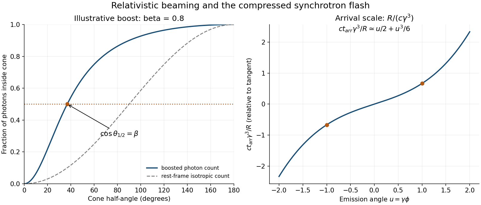
Choose the source motion along $+x$, write $\beta =v/c$, and let primes denote its instantaneous rest frame. A photon with rest-frame energy $E^{\prime }$ and direction ${\theta }^{\prime }$ has $p_x^{\prime }=E^{\prime }\cos {\theta }^{\prime }/c$ and transverse momentum $E^{\prime }\sin {\theta }^{\prime }/c$. A Lorentz boost to the laboratory givesSince $|\mathbf{p}|=E/c$, the relativistic aberration relation and its inverse areThe mapping is monotone. The boundary of the rest-frame forward hemisphere, $\cos {\theta }^{\prime }=0$, therefore maps to $\cos \theta =\beta$. An isotropic photon count assigns exactly half the photons to that hemisphere, provingThe photon count inside a relativistic beaming cone concerns an emitted ensemble and counts photons, not their total energy or the arrival-time-weighted power at a detector. The laboratory photon energies depend on direction, so “half the photons” need not mean half the radiated energy. At large $\gamma$ the angular scale is ${\theta }_{1/2}\simeq 1/\gamma$.

For a Lorentz boost of speed $v$ along $x$, the velocity-addition formula formulas areSubstitute $u_x=u\cos \theta$, $u_y=u\sin \theta$ and take the ratio. The common time-transformation denominator cancels, yieldingTo specify the direction rather than just its tangent, use ${\theta }^{\prime }=atan2(u\sin \theta /{\gamma }_v,u\cos \theta -v)$. This keeps the correct quadrant when the boost reverses the sign of the longitudinal velocity. For physical subluminal speeds the canceled denominator is positive. At $u_x=v$ and nonzero $u_y$, the transformed direction is perpendicular to the boost; if the particle is exactly comoving, its transformed velocity vanishes and the angle is undefined.

Three useful observational phenomena are relativistic Doppler effect in spectral lines from approaching and receding ejecta, relativistic beaming through jet brightness asymmetry, and apparent superluminal motion inferred from successive radio images of moving knots. The first compares spectral frequencies with rest-frame lines; the second compares the two sides after accounting for intrinsic emission and absorption; the third tests the light-travel-time relation ${\beta }_{\mathrm{app}}=\beta \sin \vartheta /(1-\beta \cos \vartheta )$. NRAO's time sequence of Galactic microquasar ejecta gives a concrete example of the third measurement.^[ref]

These are tests of relativistic radiation kinematics when source geometry and environmental effects are controlled, rather than claims that any one redshift or brightness contrast by itself uniquely proves special relativity.

For the frequency transformation, a photon has wave four-vector $K=(\omega /c,\mathbf{k})$ with $|\mathbf{k}|=\omega /c$ in vacuum. The temporal component of a Lorentz boost isThis is the relativistic Doppler effect: frequency changes both because of relative motion along the ray and because clocks in relative motion are time dilated. The angle here is measured in S. A frame chasing the photon redshifts it, ${\omega }^{\prime }/\omega =\sqrt{(1-\beta )/(1+\beta )}$; a head-on frame blueshifts it. Transverse angles defined in different frames must not be interchanged.

For the standard passive Lorentz boost, write $\beta =v/c$ andA proper orthochronous Lorentz transformation preserves the sign of the time component of a nonzero future causal vector and preserves its Minkowski norm. ThereforeThe upper-right panel of part c uses $x^{\prime }$ horizontally and $c{t}^{\prime }$ vertically. Its null rays still have slopes $\pm 1$. The grey dashed old axes satisfy $x^{\prime }=-\beta c{t}^{\prime }$ for the old time axis and $c{t}^{\prime }=-\beta x^{\prime }$ for the old spatial axis; changing the coordinate grid has not changed which events are reachable.

Use the inverse standard Lorentz boost, $t={\gamma }_v(t^{\prime }+v{x}^{\prime }/c^2)$ and $x={\gamma }_v(x^{\prime }+v{t}^{\prime })$. Label two rod endpoints by a separation $\Delta x^{\prime }=L$; their world lines satisfy $y^{\prime }=u{t}^{\prime }$. A rod's orientation in $S$ must compare endpoint events simultaneous in $S$, not in $S^{\prime }$. ConsequentlyThenThe signed counterclockwise angle therefore satisfiesFor positive $u,v$, the rod slopes downward to the right, so the acute clockwise angle is $\arctan ({\gamma }_{v}uv/c^2)$. This is a relativity of simultaneity effect in addition to the longitudinal length contraction; the rod is not being mechanically bent by the coordinate change.

Write $\Gamma =(1-v^2/c^2{)}^{-1/2}$ for the Lorentz factor of the inertial frame $S^{\prime }$, distinguishing it from the particles' changing Lorentz factors. Apply the Lorentz transformationto each world line in a. Both particles initially have velocity $-v$ in $S^{\prime }$. The switching events have coordinatesThus the Positron starts accelerating earlier in $S^{\prime }$. Its velocity first becomes less negative, vanishes when its laboratory velocity reaches $v$, and then becomes positive. The electron continues at $-v$ until $t^{\prime }=0$, then accelerates toward $-c$. The relativistic velocity-addition formula makes this precise:The electric field parallel to the Lorentz boost has unchanged magnitude, but its switching surface is $t^{\prime }+v{x}^{\prime }/c^2=0$, rather than $t^{\prime }=0$ everywhere.

In the laboratory, the total three-momentum is zero for all $t$: the two Lorentz forces cancel at equal laboratory times. In $S^{\prime }$, each active force is still $qE$, since this is one-dimensional motion with a parallel electric field. Define $t_p^{\prime }=-\Gamma vd/c^2$. For $v>0$ the total three-momentum, evaluated at equal $t^{\prime }$, isThis follows by integrating $d{p}_p^{\prime }/d{t}^{\prime }=F$ from its switching event and $d{p}_e^{\prime }/d{t}^{\prime }=-F$ from its later switching event. During the interval between them only the Positron feels the prescribed electric field, so momentum conservation for the particle pair fails. Once both forces act, the total three-momentum is constant again.

The equal-time momentum of an externally driven particle pair illustrates a distinction. The sum of particle four-momenta at a fixed pair of events is always a four-vector. However, a fresh sum at equal time in each inertial frame generally uses different events. Here transforming an equal-$t$ laboratory sum would give $-2\Gamma v\sqrt{m^2{c}^4+F^2{c}^2{t}^2}/c^2$, which varies with $t$; this differs from the equal-$t^{\prime }$ answer above. For example, with $c=m=F=d=1$ and $v=0.6$, the late-time equal-$t^{\prime }$ sum is $-0.75$, whereas transforming the equal-$t=0$ sum gives $-1.5$. This is a concrete failure of treating the pair's equal-time sums as components of a single frame-independent four-vector.

A closed system's total four-momentum, including the electromagnetic field and the apparatus supplying it, is conserved and independent of the choice of spacelike integration surface under the usual isolated-system boundary conditions. The particles alone exchange energy and momentum with an external system, so neither that independence nor universal particle-only momentum conservation is guaranteed.

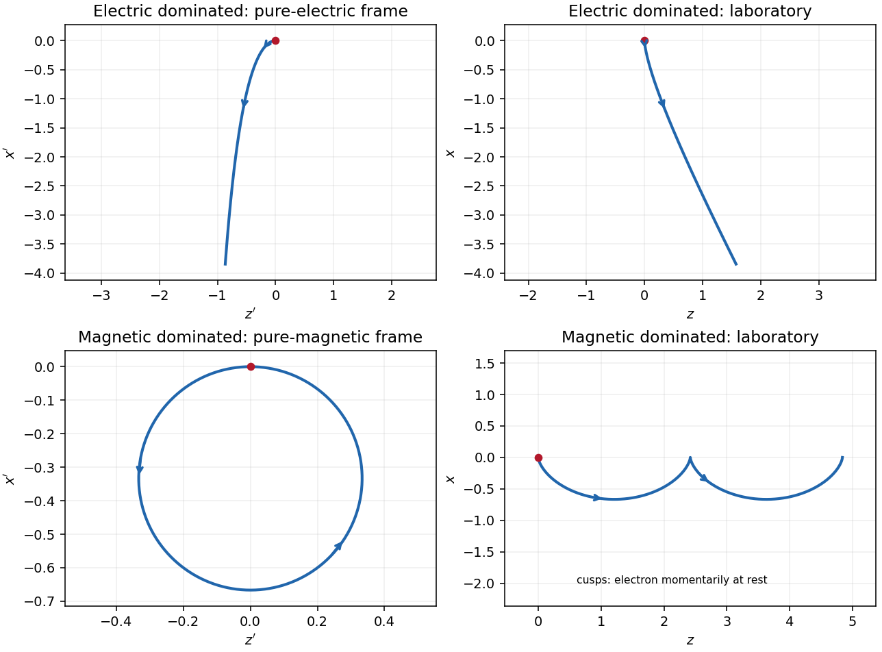
In the magnetic-dominated case the suitable Lorentz boost instead hasThe hypothesis gives $|w|<c$. The electromagnetic field invariants now have $E^2-c^2{B}^2<0$, allowing a purely magnetic inertial frame. The initial velocity is again $-w\hat{\mathbf{z}}$, perpendicular to ${\mathbf{B}}^{\prime }$. Since a magnetic field does no work, the electron's relativistic energy and speed in this inertial frame remain constant. Its trajectory is a circle in the $x^{\prime }{z}^{\prime }$ plane with Lorentz factor ${\gamma }_w$ and cyclotron frequency $\Omega =e{B}^{\prime }/({\gamma }_{w}m)$.

For $E,B>0$, set $\theta =\Omega t^{\prime }$ and $\rho =w/\Omega$. A parametrization with the correct initial velocity and Lorentz force isTransforming the world line back to the laboratory givesThe laboratory trajectory is a stretched cycloid, with cusps at $\theta =2\pi n$ where the electron is momentarily at rest. It first accelerates toward $-x$, then curves toward $+z$, returning to its original $x$ coordinate each cycle while advancing in $z$. Its mean drift is $\Delta z/\Delta t=w=E/B$, the E-cross-B drift. Its laboratory kinetic energy oscillates as the electric field does positive and then negative work; it does not grow indefinitely. The strict inequalities in the two branches exclude the null case $|E/B|=c$, where neither field can be removed by a finite Lorentz boost.

Assume $E,B>0$ for the directions and parametrizations; the boost formulas retain their signed meaning for reversed fields. A Lorentz boost with velocity $w\hat{\mathbf{z}}$ along $\mathbf{E}\times \mathbf{B}$ transforms the transverse electric field and magnetic field asIn the electric-dominated case chooseThe inequality ensures $|w|<c$, so this is an inertial frame. The field-removing boosts for perpendicular electric and magnetic fields are governed by the electromagnetic field invariants $\mathbf{E}\cdot \mathbf{B}=0$ and $E^2-c^2{B}^2>0$ explain why a purely electric inertial frame exists and a purely magnetic one does not.

The electron is not initially at rest in this convenient inertial frame: its initial velocity is $-w\hat{\mathbf{z}}$ and its initial three-momentum is $p_z^{\prime }=-{\gamma }_{w}mw$. Thereafter $p_x^{\prime }=-e{E}^{\prime }{t}^{\prime }$, while $p_z^{\prime }$ stays constant. The electric field accelerates it toward $-x$; as its relativistic energy increases, its negative transverse velocity decreases in magnitude. Defining $a=e{E}^{\prime }/m>0$ and $s=a\tau /c$ gives a useful parametric world line:Here $\tau$ is the proper time. These formulas follow by integrating $U^{\prime 0}={\gamma }_{w}c\cosh s$, $U^{\prime x}=-{\gamma }_{w}c\sinh s$, and constant $U^{\prime z}=-{\gamma }_{w}w$. Its projection onto the $t^{\prime },x^{\prime }$ plane is a hyperbola, but the spatial trajectory includes the initial transverse motion and is not a straight line.

Transforming back with $z={\gamma }_w(z^{\prime }+w{t}^{\prime })$, $t={\gamma }_w(t^{\prime }+w{z}^{\prime }/c^2)$ givesThe laboratory trajectory starts from rest toward $-x$, then bends toward $+z$. It is unbounded in $-x$ and ultimately has $u_z\to w=c^{2}B/E$ and $u_x\to -c/{\gamma }_w$. Thus the late velocity has magnitude $c$ as a limit, consistent with the relativistic energy-momentum relation, rather than undergoing a closed cyclotron orbit.

Let starred quantities denote the capacitor's rest inertial frame, $u_0={ϵ}_0{E}^2/2$, $\beta =v/c$, and $\gamma =(1-{\beta }^2{)}^{-1/2}$. Work in the uniform interplate region of an ideal parallel-plate capacitor, neglecting its fringing field of a capacitor. To transform from that rest inertial frame to a laboratory in which the capacitor moves along $+x$, use the positive-sign Lorentz transformationFor a purely electric field, the spatial block of the electromagnetic stress-energy tensor isThis is the negative of the Maxwell stress tensor: it has $-u_0$ along the electric field and $+u_0$ perpendicular to it. The stress contribution to energy transport in a moving capacitor is essential to the Lorentz transformation of the energy density and flux.

Plates parallel to $xy$. Choose ${\mathbf{E}}_{\ast }=E\hat{\mathbf{z}}$ and ${\mathbf{B}}_{\ast }=0$. The electromagnetic field tensor and electromagnetic stress-energy tensor areThe transformed nonzero independent electromagnetic field tensor components are $F^{03}=\gamma E/c$ and $F^{13}=\gamma \beta E/c$. Thus $\mathbf{E}=\gamma E\hat{\mathbf{z}}$ and $\mathbf{B}=-\gamma vE\hat{\mathbf{y}}/c^2$, consistent with $\mathbf{B}=\mathbf{v}\times \mathbf{E}/c^2$. Transforming the electromagnetic stress-energy tensor givesIn particular, the laboratory Poynting vector is $\mathbf{S}=2u_0{\gamma }^{2}v\hat{\mathbf{x}}$, and the electromagnetic energy density is $u=u_0{\gamma }^2(1+{\beta }^2)$. The ratio $S_x/u=2v/(1+{\beta }^2)$ is subluminal for $v<c$, but differs from the capacitor's velocity. The difference from a simple convective flux isThe extra term is $v{T}_{\ast }^{xx}$, the rest-frame stress multiplied by the velocity. This shows why treating stored field energy as an unstressed parcel moving rigidly with the plates misses part of the energy transport.

Plates parallel to $yz$. Now ${\mathbf{E}}_{\ast }=E\hat{\mathbf{x}}$. The rest tensors areThe electric field is parallel to the Lorentz boost, so $F^{01}=E/c$ remains unchanged and $\mathbf{B}=0$. The cancellation between $T_{\ast }^{00}$ and $T_{\ast }^{11}$ givesThere is no Poynting flux in the ideal interior in this orientation, although the region containing the electric field moves. The longitudinal negative stress contribution cancels the convective term: $S_x={\gamma }^{2}v(u_0+T_{\ast }^{xx})=0$. Field energy is removed at the receding boundary and supplied at the advancing boundary by work on the charged plates; it need not flow through the interior to accompany the moving region. At edges, omitted fringing fields provide additional local structure.

For a finite idealized interplate rest volume $V_0$, length contraction gives $V=V_0/\gamma$. The field-only integrated laboratory energies would consequently be $U_{xy}=\gamma (1+{\beta }^2)U_0$ and $U_{yz}=U_0/\gamma$, with $U_0=u_0{V}_0$. Their different transformation laws are not paradoxical: the field alone is not a closed system. Include the plates and the supports holding them apart, whose mechanical stresses balance the Maxwell stress tensor. The total closed-system four-momentum then has the ordinary Lorentz transformation law. This is the same distinction between a subsystem and a conserved whole that appears in b.

For an active clockwise rotation of column vectors in the usual oriented $xy$ plane, takeDirect matrix multiplication givesThus the rotation matrix is an orthogonal matrix, preserving the Euclidean inner product, with determinant $+1$.

For a passive one-dimensional Lorentz boost, use rapidity $\eta$, $\beta =\tanh \eta$:This is not $I$ unless $\eta =0$. Hence a nontrivial Lorentz boost is not an orthogonal matrix for the Euclidean inner product. Instead it preserves the Minkowski metric:by ${\cosh }^2\eta -{\sinh }^2\eta =1$. Thus it is pseudo-orthogonal. The zero-rapidity identity is the explicit exception to the assertion that a Lorentz boost is not orthogonal.

Let $K_i$ generate Lorentz boosts with the same exponential convention as the rotation generators of rotations $J_i$. The Lie algebra of the Lorentz group isConsequently non-collinear Lorentz boosts do not close among themselves: the product contains a rotation, the Wigner rotation. For an explicit counterexample, in coordinates $(ct,x,y)$ write $c_a=\cosh a$, $s_a=\sinh a$ and similarly for $b$. ThenA pure rotationless Lorentz boost has a symmetric matrix, whereas this product has spatial entries $(xy)=0$ and $(yx)=s_a{s}_b\ne 0$ for $a,b\ne 0$. It is therefore a concrete product of two pure Lorentz boosts that is not a pure Lorentz boost. Collinear Lorentz boosts are the special case that do form a one-parameter group, with additive rapidities.

Allowing all spatial directions and closure generates both the $K_i$ and, through their commutators, all $J_i$. The smallest connected group containing all these Lorentz boosts is the proper orthochronous Lorentz groupIt contains arbitrary compositions of spatial rotations and Lorentz boosts continuously connected to the identity. It has six continuous parameters. Here “smallest” refers to the subgroup generated by all continuous pure Lorentz boosts, not to an arbitrary collection already including discrete reversals.

The full Lorentz group $O(1,3)$ has four connected components, distinguished by the sign of the determinant and the direction of time. Representatives are the identity, parity $P=\mathrm{diag}(1,-1,-1,-1)$, time reversal $\mathsf{T}=\mathrm{diag}(-1,1,1,1)$, and $P\mathsf{T}=-I$. ThusMultiplication by these discrete transformations relates the components algebraically; no continuous path within the Lorentz group joins different components. Translations are not required for closure here; adding them gives the larger Poincaré group.

Write the Lorentz transformation as $x^{\prime \mu }={\Lambda }^{\mu }{}_{\nu }{x}^{\nu }$. Acting on a scalar field, the chain rule gives the four-gradientFor the specified Lorentz boost, the inverse is obtained by changing $\beta$ to $-\beta$, soThese are precisely the covector component rules for the lowered coordinates. Raising the index with the Minkowski metric ${\eta }^{\mu \nu }=\mathrm{diag}(-1,1,1,1)$ reverses the time component, yieldingIndeed ${\partial }^{\prime 0}=\gamma ({\partial }^0-\beta {\partial }^1)$ and ${\partial }^{\prime 1}=\gamma ({\partial }^1-\beta {\partial }^0)$, the contravariant four-vector rules. Thus the index on a partial derivative with respect to an upper coordinate is lower.

Use $c=1$ and define the total four-momentum $P^{\mu }=(E,\mathbf{P})={\sum }_i(E_i,{\mathbf{p}}_i)$. For an inertial frame moving with velocity $\mathbf{V}$ relative to the laboratory, the Lorentz boost givesChoose $\mathbf{V}$ parallel to $\mathbf{P}$ and require zero total three-momentum. ThenThis requires $E>|\mathbf{P}|$, so that the total four-momentum is timelike. Its invariant mass is $\sqrt{E^2-|\mathbf{P}{|}^2}$, the total relativistic energy in the center-of-momentum frame. If all particles are exactly parallel photons, the total four-momentum is null and no finite-velocity center-of-momentum frame exists.

Sign qualification. The minus sign printed in the source describes the laboratory's velocity in the center-of-momentum frame, or the parameter of an active Lorentz boost with a plus-sign spatial rule. It is not the velocity of the center-of-momentum frame relative to the laboratory under question 1's passive convention. For example, a single particle with $(E,P_x)=(5,3)$ has its rest frame moving at $V_x=3/5$. The printed $V_x=-3/5$ would give $P_x^{\prime }=(5/4)(3+3)=15/2$, which is not zero. This explicitly resolves the sign rather than assigning a rest frame moving away from the particle.

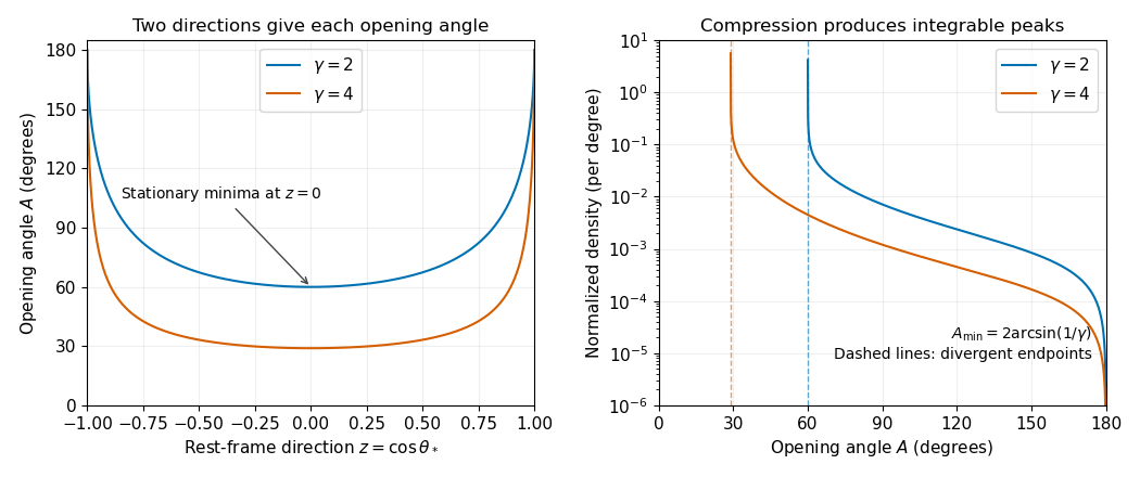
In the center-of-momentum frame, four-momentum conservation gives two opposite photon momenta, each of energy $M_{\pi }/2$. Let $z=\cos {\theta }_{\ast }$, with the axis along the Lorentz boost from that frame to the laboratory. Reversing the axis specified in the source changes $z$ to $-z$ and has no effect on the following product. The Lorentz transformation of four-momentum givesWriting $s=\sin (A/2)$, b now impliesThe isotropy assumption is $dN=a|dz|$ on $-1\le z\le 1$. Each interior opening angle has two inverse branches, $z$ and $-z$, both of which must enter the change of variables for probability densities. The positive branch has derivativeConsequently the diphoton opening-angle distribution isIts support is $2\arcsin (1/\gamma )<A<\pi$ for $0<\beta <1$, and its integral is $2a$, the integral of the original angular probability density before normalization. Thus the normalized probability density is $(2a{)}^{-1}dN/dA$. Omitting one inverse branch would incorrectly halve the total count.

From c, $\sin (A/2)\ge 1/\gamma$, with equality when $z=0$: the photons are emitted perpendicular to the Lorentz boost axis in the center-of-momentum frame. ThereforeAt the minimum, the map $z\mapsto A$ is stationary: writing $A=A_{\min }+\delta$, its leading behavior is $\delta =\beta z^2/\gamma +O(z^4)$. A nonzero interval of uniformly distributed $z$ is therefore compressed near $A_{\min }$, producing an integrable inverse-square-root singularity in the opening-angle probability density. No differentiation of that probability density is needed. For finite $\gamma >1$, the probability density vanishes at $A=\pi$. For $\gamma =1$ the center-of-momentum frame is the laboratory and every event has $A=\pi$: the probability distribution becomes a Dirac delta distribution, rather than the singular $\beta =0$ substitution in c. At large $\gamma$, $A_{\min }\sim 2/\gamma$ in radians.

The Lorentz boost from A to B givesDivide each spatial displacement by $d{t}^{\prime }={\gamma }_{v}dt(1-v{u}_x/c^2)$. The velocity-addition formula isThe same result follows by transforming the four-velocity and using $w_i=c{U}^{\prime i}/U^{\prime 0}$. The transverse velocities change because the transformed time increment depends on $dx$, even though the transverse spatial coordinates are unchanged.

For $v=|\mathbf{v}|>0$, decompose the velocity as $\mathbf{u}={\mathbf{u}}_{\parallel }+{\mathbf{u}}_{\perp }$, parallel and perpendicular to $\mathbf{v}$. A rotation-free Lorentz boost gives the velocity-addition formulaThese two components are orthogonal, soThe last equality is Lagrange's identity for the cross product. For physical subluminal speeds, $D>0$, givingThe $\mathbf{v}=0$ case follows directly or by continuity. An independent form useful for checks is $1-|\mathbf{w}{|}^2/c^2=(1-u^2/c^2)(1-v^2/c^2)/D^2$, obtained from the transformed four-velocity normalization.

Use the amplitude placement in the original PDF: $w=[A{\cosh }^2(Bx){]}^{1/(1-n)}$. Introduce the actual peak $C=A^{-1/(n-1)}$ and $p=2/(n-1)$, so $w=C{\mathrm{sech}}^p(Bx)$. Its derivatives satisfyThe static equation is $w^{\prime \prime }=aw-b{w}^n$. Matching the constant and ${\mathrm{sech}}^2$ terms givesChanging the sign of $B$ leaves the profile unchanged. If $A$ is instead defined as an outside prefactor, as in the held TeX transcription, its value is $C$, not the PDF's $A$. This notation discrepancy does not change the physical profile.

The nonconstant positive power-law nonlinear Klein-Gordon pulse is even, smooth, has peak $C$ at zero and decays as $e^{-\sqrt{a}|x|}$. The requested sketches below compare several powers with illustrative $a=b=1$. For odd $n$, its negative is also a solution. A separate constant branch occurs for $B=0$: the positive equilibrium has $C=(a/b{)}^{1/(n-1)}$, or $A=b/a$ in the PDF convention. The zero solution is another equilibrium, obtained as a limiting profile rather than finite positive $A$.

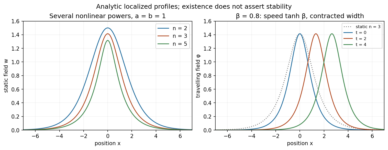
Now apply the Lorentz boost with rapidity $-\beta$ to the static field. It givesFor positive $\beta$, the centre moves to the right at $0<v<1$, with speed one the wave-speed unit. The peak stays $C$ and the width contracts by $1/\cosh \beta$. The shape translates without changing in time. This establishes a travelling solitary pulse; it does not by itself prove stability or elastic multi-pulse scattering.