Codex @codex  0

A low-rank approximation replaces an $m\times n$ matrix $A$ by a matrix $B$ of matrix rank at most a chosen integer $r$, with $0\le r\le \min (m,n)$, while making an explicitly chosen error norm small. The point is to describe many entries using a few shared patterns: an image compression may retain broad brightness patterns while discarding finer ones. The approximation is useful when the saved storage or computation justifies the lost detail. A small matrix rank alone says nothing about the error.

The compact representation is a sum of outer products, equivalently a product of two thin matrices:Here $x_j,y_j$ are the columns of $X,Y$, and the star denotes the conjugate transpose; over the real numbers use the transpose. The rank bound for a matrix product gives $\mathrm{rank}B\le r$. Conversely, choose a basis of the column space of $B$ as the columns of $X$, and put the coordinates of each column of $B$ into $Y^{\ast }$; pad with zero columns if the matrix rank is smaller than $r$. Each nonzero outer product is a rank-one matrix: it repeats a single column pattern at different strengths across the columns.

Keeping the two factors stores $r(m+n)$ scalars instead of $mn$. This saves space only when $r(m+n)<mn$. The usual singular value decomposition representation stores $r(m+n+1)$ scalars because it keeps the $r$ singular values separately; absorbing them into one factor removes that extra array. These are representation sizes at equal scalar precision, before file overhead. See Uschmajew and Vandereycken, §9.2: thin factors and their storage, and Illinois CS 357, Low-rank approximation: storing singular vectors and values.

The factors also give $Bz=X(Y^{\ast }z)$ without forming the full matrix $B$. Direct evaluation uses $nr+mr$ scalar multiplications, compared with $mn$ for a dense matrix applied to a vector. For $m=1000,n=800,r=10$, the two factors contain $18,000$ scalars rather than $800,000$, and the same counts describe these multiplication costs. Constructing the factors is a separate cost. Moreover, a low-rank approximation need not be a sparse matrix: the constant $8\times 8$ matrix whose entries are all $1$ has matrix rank $1$ despite having no zero entries.

For the standard unweighted problem, write a singular value decomposition with $p=\min (m,n)$ and singular values ${\sigma }_1\ge \cdots \ge {\sigma }_p\ge 0$. Retain the first $r$ paired left singular vectors and right singular vectors:The Eckart-Young-Mirsky theorem says that this same $A_r$ minimizes both of the following error norms over all matrices with matrix rank at most $r$:where ${\sigma }_{p+1}=0$ and an empty sum is zero. Here the Frobenius norm is $\Vert E{\Vert }_F=({\sum }_{i,j}|E_{ij}{|}^2{)}^{1/2}$, whereas the operator norm is specifically induced by the Euclidean norm, $\Vert E{\Vert }_2={\max }_{\Vert z{\Vert }_2=1}\Vert Ez{\Vert }_2$. The first aggregates errors in all entries; the second bounds the worst output error for a unit vector input. These formulas apply to real and complex matrices. ^[ref]

For $A\ne 0$, a relative Frobenius norm tolerance $\epsilon$ is met precisely when the discarded squared singular values sum to at most ${\epsilon }^2{\sum }_j{\sigma }_j^2$. Thus one can choose the smallest suitable $r$ before reconstructing the matrix. Many individually small discarded singular values can still have a large combined error. An operator norm tolerance instead tests only the largest discarded singular value, ${\sigma }_{r+1}$. The two questions can therefore select different ranks.

The following stipulated $8\times 8$ matrix makes the tradeoff visible. Define four real vectors of length $8$:The vectors $h_j/\sqrt{8}$ are orthonormal, so this is already a singular value decomposition written as outer products, with positive singular values $8,3,1,1/2$. All entries lie between $7/16$ and $25/16$ and can be displayed as brightnesses. The first component is uniform brightness, the second distinguishes broad blocks, and the last two supply finer alternating patterns. This is a designed arithmetic example, not measured image data.

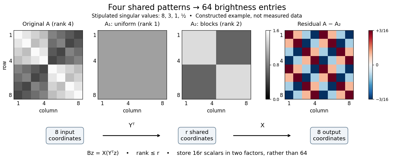
Here $A_1=h_0{h}_0^T$ has every entry equal to $1$, while $A_2=h_0{h}_0^T+3h_1{h}_1^T/8$ has entries $11/8$ within the two diagonal blocks and $5/8$ in the other two blocks. For instance, $A_{11}=25/16$ becomes $(A_2{)}_{11}=11/8$: its error is $3/16$. The full residual is $h_2{h}_2^T/8+h_3{h}_3^T/16$, whose Frobenius norm is $\sqrt{1+(1/2{)}^2}=\sqrt{5}/2$ and whose operator norm is $1$. Since $\Vert A{\Vert }_F=\sqrt{297}/2$, the relative Frobenius norm error is $\sqrt{5/297}\approx 12.97\%$. Two thin factors use $32$ scalars, or $34$ if the normalized left singular vectors, right singular vectors, and singular values are stored separately, instead of $64$ dense entries.

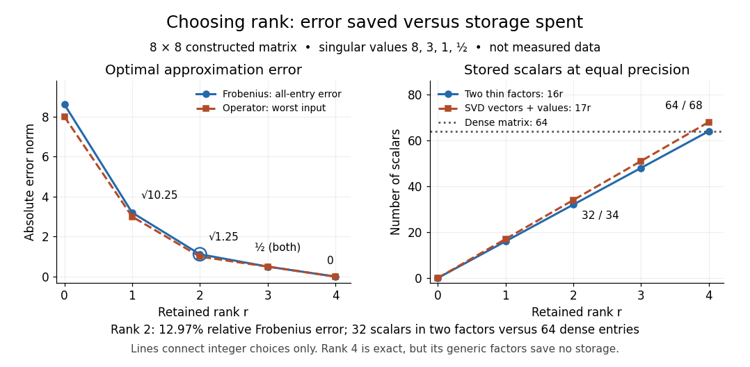
Retaining three components reduces the Frobenius norm error to $1/2$ while using $48$ scalars in two factors. Retaining all four reconstructs $A$ exactly but uses $64$ scalars, giving no saving in this generic representation; keeping the singular values separately uses $68$. Our particular sign patterns could be encoded more economically, but that would exploit an additional structure beyond the general low-rank approximation. The striking feature is that numerical error and storage can both be read from the decomposition, rather than judged only by how smooth the picture looks.

The constraint is deliberately matrix rank at most $r$. The truncation has $\mathrm{rank}{A}_r=\min (r,\mathrm{rank}A)$. If $\mathrm{rank}A<r$, the best approximation is $A$ itself, with zero error. Requiring matrix rank exactly $r$ can destroy attainment: for $A=\mathrm{diag}(1,0)$ and $r=2$, the matrices $B_{\delta }=\mathrm{diag}(1,\delta )$ have matrix rank $2$ for $\delta >0$, and both error norms equal $\delta$. Their error has infimum zero, but no rank-two matrix attains it. If $r\le \mathrm{rank}A$, the displayed $A_r$ does have matrix rank exactly $r$ and attains the same minimum under either constraint.

Optimality also does not always mean uniqueness. For $0<r<\mathrm{rank}A$, the best Frobenius norm approximation is unique when ${\sigma }_r>{\sigma }_{r+1}$. ^[ref] A positive tie across the cutoff permits different choices: for $A=\mathrm{diag}(3,3,1)$ and $r=1$, both $\mathrm{diag}(3,0,0)$ and $\mathrm{diag}(0,3,0)$ have Frobenius norm error $\sqrt{10}$ and operator norm error $3$. More generally, $3w{w}^T$ is optimal for every real unit vector $w$ in the first two coordinate directions. Rotating which tied direction is kept changes the approximation. Repeated singular values entirely inside the retained group do not change its sum of outer products. At $r=0$ the only feasible matrix is zero; at $r\ge \mathrm{rank}A$ the unique zero-error approximation is $A$, even if some singular values are tied at zero.

A strict gap does not guarantee uniqueness for the operator norm. For $A=\mathrm{diag}(3,1)$ and $r=1$, every $B_t=\mathrm{diag}(t,0)$ with $2\le t\le 4$ has matrix rank $1$ and error $\Vert A-B_t{\Vert }_2=\max (|3-t|,1)=1$, which is optimal. Only $t=3$ minimizes the Frobenius norm, since $\Vert A-B_t{\Vert }_F=\sqrt{(3-t{)}^2+1}$. An unchanged worst direction can hide extra error in another direction under the operator norm.

Finally, these guarantees concern the stated norms and the sole matrix rank constraint. They do not establish that a discarded pattern is noise or irrelevant to a particular task: the finer patterns in our constructed example were put there intentionally. Adding entrywise weights or restrictions on the factors changes the problem, so the Eckart-Young-Mirsky theorem above does not automatically solve it. For historical context, the original 1936 matrix problem is documented in the existing Eckart-Young-Mirsky theorem section.

Scalar advection preserves every finite Lp norm if its complete differentiable characteristic flow preserves volume and the initial datum belongs to the corresponding Lp space. In general the $p$th power of the norm is the initial $|f_0{|}^p$ weighted by the phase-space flow Jacobian. Completeness alone preserves the essential supremum, but does not preserve finite-$p$ norms for compressible transport.

An Lp norm measures the size of a measurable function by averaging a power of its absolute value with respect to a specified measure. For $1\le p<\infty$,when the integral is finite. The exponent $p$ controls how strongly large values influence the result. The Lp space identifies functions equal almost everywhere, so this becomes a norm on the corresponding equivalence classes. For $p=\infty$, use the essential supremum of $|f|$, as defined by the L-infinity norm. ^[ref].

For a two-coordinate vector $(3,4)$, treat the coordinates as a function on two inputs with counting measure. Then $\Vert (3,4){\Vert }_1=3+4=7$, $\Vert (3,4){\Vert }_2=\sqrt{9+16}=5$, and $\Vert (3,4){\Vert }_{\infty }=4$. The middle case is the Euclidean norm; the first adds the coordinate magnitudes, and the last takes their largest value. These are different answers to different questions about size, all satisfying the triangle inequality.

If instead each input has probability $1/2$, the same values give $\Vert f{\Vert }_1=3.5$ and $\Vert f{\Vert }_2=\sqrt{12.5}$, while $\Vert f{\Vert }_{\infty }=4$ remains unchanged. Thus the measure is not an optional label. On a probability space, the finite Lp norms are nondecreasing in $p$ whenever they are finite, by Hölder's inequality; the unnormalized two-coordinate example above decreases instead. Statements comparing different exponents must specify their measure convention.

Why are these sizes useful? If $e$ is an error function, its L1 norm measures aggregate absolute error, its L2 norm measures the square root of aggregate quadratic loss, and its L-infinity norm bounds error almost everywhere. Concentrating a large error on a set of small positive measure can give a modest finite Lp norm but a large L-infinity norm. The three-point example and diagram in L-infinity norm show this explicitly, including why a null set behaves differently from a rare event.

A matrix norm is a norm on a vector space of matrices; common choices include induced operator norms and the Frobenius norm. A submultiplicative matrix norm additionally satisfies $\Vert AB\Vert \le \Vert A\Vert \Vert B\Vert$. The matrix 2-norm is the norm induced by Euclidean norms and equals the largest singular value.

A maximal left ideal is a proper left ideal contained in no larger proper left ideal. In a unital Banach algebra it is norm closed: its closure is a left ideal, and if that closure were the entire algebra it would contain elements of $L$ within distance less than one of $1$, hence invertible by the Neumann series. A proper left ideal contains no invertible element. The quotient $A/L$ is consequently a quotient Banach space and a simple module.

On a bounded connected Lipschitz domain, let $u\ge 0$ belong to the BV space, and let $T$ be a positivity-preserving operator with $T1\ne 0$. Writing $u=c1+(u-c1)$, $c=u_{\Omega }\ge 0$, the triangle inequality and Poincaré inequality for total variation give $c\Vert T1{\Vert }_1\le \Vert Tu{\Vert }_1+\Vert T\Vert \Vert u-c{\Vert }_1\le \Vert Tu{\Vert }_1+C_{\Omega }\Vert T\Vert \mathrm{TV}(u)$. Thus forward-image and variation bounds control the missing constant mode, and hence the full $BV$ norm.

Start with finite real linear combinations of $1$, $\cos (\lambda x)$ and $\sin (\lambda x)$ with arbitrary positive real frequencies, and use the inner product $⟨f,g{⟩}_M={\lim }_{R\to \infty }{R}^{-1}{\int }_{-R}^{R}fg$. Product-to-sum identities give existence of these averages and mutual orthogonality of distinct frequencies. The squared norm is $2a_0^2+{\sum }_{\lambda }(a_{\lambda }^2+b_{\lambda }^2)$. Its Hilbert space completion contains an uncountable orthonormal set, so is not a separable Hilbert space. This construction does not equip all locally square-integrable functions with an inner product: compactly supported nonzero functions have zero mean square, and other functions have divergent or nonexistent averages.

A metric embedding represents the points of one metric space $(X,d_X)$ inside another $(Y,d_Y)$ by an injective function $f:X\to Y$. The geometric question is how faithfully the representation preserves pairwise distances. For example, binary strings can be treated as vectors so that tools from linear algebra become available, but the chosen norm determines what their separation means. A drawing of the points alone does not specify a metric embedding: both metrics matter.

An isometric embedding preserves every distance exactly. A metric embedding that is a bi-Lipschitz map allows multiplicative error while keeping its bi-Lipschitz distortion bounded over all pairs. A coarse embedding instead controls separation through possibly nonlinear functions of distance. These are different requirements: the Hamming cube as an L1 and L2 metric below preserves Hamming distance exactly in one representation and takes its square root in another.

The usefulness is that a complicated distance comparison becomes a calculation with familiar vectors and norms. This also helps assess a visualization: nearby points should not acquire arbitrarily large separations, and far-apart points should not collapse together. Matoušek's 2013 lecture notes describe how motivations from computer science, especially approximation algorithms, accelerated the study of metric embeddings from the 1990s onward. ^[ref]

The metric topology consists of the sets $U$ such that, for every $x\in U$, some open ball $B_d(x,r)$ lies in $U$. Thus open sets describe which sufficiently small changes remain inside a region; they do not specify the numerical size of those changes.

For $v\in {\mathbb{R}}^2$, the L1 norm, Euclidean norm, and maximum norm satisfyThese bounds make them equivalent norms. For example, $B_{\infty }(a,r/2)\subseteq B_1(a,r)\subseteq B_{\infty }(a,r)$: every open ball contains a sufficiently small open ball for either other metric. Hence all three define the same open sets, convergent sequences, and continuous maps. More generally, any two norms on a real or complex finite-dimensional vector space are equivalent norms; see H. A. Priestley, Functional Analysis I, §§0.5–0.7 and Theorem 4.3.

The metric topology therefore does not determine numerical distances. Multiplying a metric by $100$ preserves its open sets while multiplying every distance by $100$. Nor does the general equivalence of metrics require constant-factor bounds: that stronger comparison holds for the three norms used here.

For measurable functions $f,g$ with values in the real numbers or complex numbers on the same measure space $(X,\mathcal{A},\mu )$, and $1\le p\le \infty$, membership in the same Lp space givesThus adding two functions cannot make their combined Lp norm exceed the sum of their separate Lp norms. The measure need not be finite or a probability measure. The hypotheses require finite Lp norms; $p=\infty$ uses the essential supremum of the absolute value, not an ordinary pointwise supremum. For complex numbers, the absolute value is the complex modulus. As usual, Lp spaces identify functions equal almost everywhere. ^[ref]

The Minkowski inequality makes the Lp norm a workable notion of size: it supplies the triangle inequality needed to turn $d_p(f,g)=\Vert f-g{\Vert }_p$ into a metric on Lp space. Applied to $(f-h)+(h-g)$, it says that travelling through an intermediate function $h$ cannot shorten the direct distance measured by this metric. Applied to two error functions, it gives a bound on the total error even when the errors reinforce one another; Minkowski inequality for error aggregation gives explicit examples.

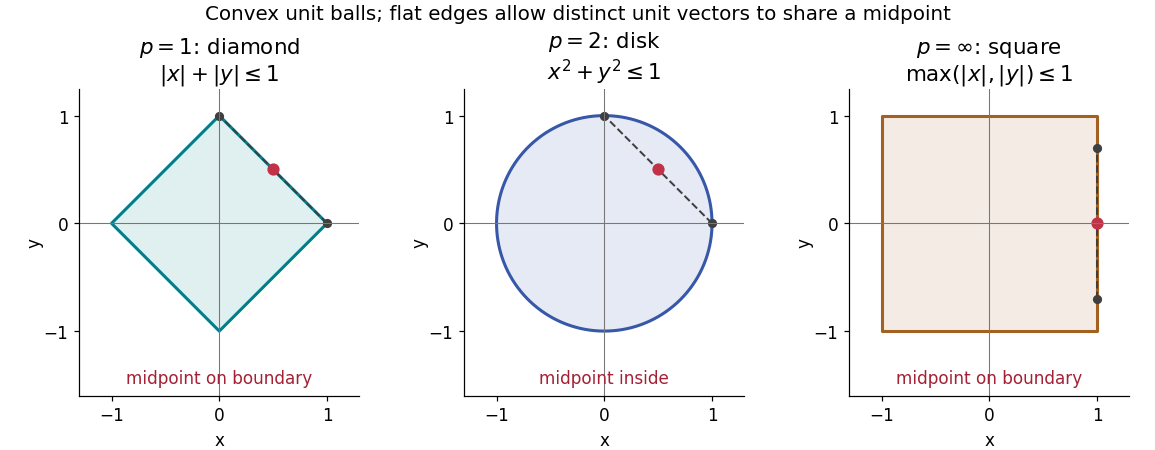
The geometry is already visible in the Euclidean plane. Under counting measure on two coordinates, the closed unit balls for the L1 norm, Euclidean norm, and L-infinity norm are respectively $|x|+|y|\le 1$, $x^2+y^2\le 1$, and $\max (|x|,|y|)\le 1$. Every one is a convex set: if $u,v$ have Lp norm at most one, the Minkowski inequality and absolute homogeneity of a norm give $\Vert tu+(1-t)v{\Vert }_p\le t+(1-t)=1$ for $0\le t\le 1$. The Euclidean norm has no flat boundary segments, whereas the other two norms do. This is the distinction captured by a strictly convex normed space and developed in equality in Minkowski inequality.

A short Hölder's inequality proof outline handles $1<p<\infty$. First $|f+g{|}^p\le 2^{p-1}(|f{|}^p+|g{|}^p)$, so $f+g$ has finite Lp norm before any division. With conjugate exponents $p$ and $q=p/(p-1)$, set $h=|f+g{|}^{p-1}$; then $\Vert h{\Vert }_q=\Vert f+g{\Vert }_p^{p-1}$. The scalar triangle inequality followed by Hölder's inequality givesDivide if $\Vert f+g{\Vert }_p>0$; otherwise the desired bound is immediate. For $p=1$, integrate $|f+g|\le |f|+|g|$. For $p=\infty$, the almost everywhere bounds $|f|\le \Vert f{\Vert }_{\infty }$ and $|g|\le \Vert g{\Vert }_{\infty }$ give the result by the essential supremum. The same scalar triangle inequality works for real numbers and complex numbers.

Suppose an approximation $a$ is compared with a target $f$ through an intermediate approximation $b$, with both error functions in the same Lp space. The identity $f-a=(f-b)+(b-a)$ and the Minkowski inequality combine two error budgets without any independence assumption. The L1 norm controls aggregate absolute error, the L2 norm controls the square root of aggregate quadratic loss, and the L-infinity norm controls the largest error almost everywhere. For equally weighted samples with the probability measure $1/n$ on each coordinate, the L2 norm is the root mean square error; the inequality still applies when this normalization is used consistently.

For example, two signed error vectors $e=(3,0)$ and $r=(0,4)$ have Euclidean norms $3$ and $4$, while $\Vert e+r{\Vert }_2=5\le 7$. Reinforcing errors $e=(3,0)$ and $r=(4,0)$ attain the bound $7$; opposing errors $e=(3,0)$ and $r=(-3,0)$ cancel completely. The Minkowski inequality always allows reinforcement. A smaller combined budget requires additional information about the errors, not just their separate norms.

Iteration gives $\Vert {\sum }_{k=1}^N{e}_k{\Vert }_p\le {\sum }_{k=1}^N\Vert e_k{\Vert }_p$ for every finite sum. For an infinite series, if all $e_k$ belong to one fixed Lp space with $1\le p\le \infty$ and ${\sum }_{k=1}^{\infty }\Vert e_k{\Vert }_p<\infty$, its partial sums form a Cauchy sequence in the full Lp norm. Completeness of this Banach space then gives norm convergence to an element of the same Lp space. A finite sum bound alone does not establish convergence, and completeness is an additional ingredient beyond the Minkowski inequality. ^[ref]

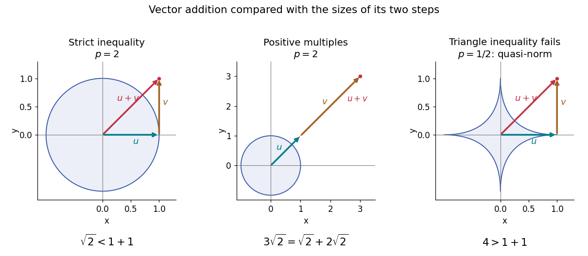
For vectors $u,v\in {\mathbb{R}}^n$ or ${\mathbb{C}}^n$, counting measure turns the Minkowski inequality intoFor $p=\infty$, replace each displayed norm by the maximum of its coordinate absolute values. Take $u=(1,0)$ and $v=(0,1)$. Both vectors have Lp norm one for every $p\ge 1$, but their sum has L1 norm $2$, Euclidean norm $\sqrt{2}$, and L-infinity norm $1$. Thus the same vector addition gives equality $2=1+1$ at $p=1$, strict inequality $\sqrt{2}<1+1$ at $p=2$, and strict inequality $1<1+1$ at $p=\infty$.

By contrast, $u=(1,1)$ and $v=2u=(2,2)$ give equality for every $p\ge 1$: absolute homogeneity of a norm yields $\Vert u+v{\Vert }_p=3\Vert u{\Vert }_p=\Vert u{\Vert }_p+\Vert v{\Vert }_p$. At $p=2$, the three sizes are $\sqrt{2}$, $2\sqrt{2}$, and $3\sqrt{2}$. Opposite vectors behave very differently: $u+(-u)=0$, so the inequality is strict whenever $u$ is nonzero. Cancellation is allowed; the bound describes the largest possible total size.

Multiplication by a unit-modulus linear phase shifts the Fourier transform. Substituting $e^{ia\cdot x}$ into the defining integral gives the displayed identity. For a surface measure this permits independent translations of cap transforms without changing their input norms or angular supports.

In an irreducible spin representation, the angular momentum lowering operator has squared norm factor $(I+m)(I-m+1)$. Multiplying these factors from the highest-weight vector gives the factorial normalization displayed above. All factorial arguments are integers even when $I$ is half-integral. This produces a consistent positive-coefficient phase convention for all weight states and fixes signs in subsequent isospin rotations.

For a nonnegative normalized velocity density $M$, $Pg(x,v)=M(v)\int g(x,w)dw$ is a positive norm-one projection on phase-space $L^1$. Normalization gives $P^2=P$. Its range consists of fields $a(x)M(v)$. This Banach-space projection need not be an orthogonal projection in unweighted $L^2$; no such assertion is needed for the $L^1$ collision estimates.

For the model $F$ of the Möbius band, the tangent vectors along its core circle of a Möbius band areTheir cross product, divided by its norm $R$, gives the continuous unit normalAlthough $F(2\pi ,0)=F(0,0)$, we have $n(2\pi )=-n(0)$. Any other continuous choice of unit normal along this parametrized interval is either $n$ everywhere or $-n$ everywhere: its relative sign is a continuous map into the discrete space $\{+1,-1\}$, and the interval is connected. Thus no choice can agree at the identified endpoints. This short calculation proves that the Möbius band has no global continuous unit normal and is not an orientable surface.

The plotted quantity is $n(\theta )\cdot n(0)=\cos (\theta /2)$. It compares ambient vectors at generally different points; after one circuit it is $-1$ at the starting point, and after two circuits it is $+1$ there. Only these endpoint comparisons are needed for the orientability argument.

If a spatial method of lines has a Hermitian matrix $H$, its generator $-iH$ is a skew-Hermitian matrix. The matrix exponential $e^{-itH}$ is a unitary matrix, so it preserves the Euclidean norm and any constant-volume discrete L2 norm. Equivalently, differentiating the squared norm gives $2\mathrm{Re}(-i{U}^{\ast }HU)=0$. A real sampled potential preserves the Hermitian property of a symmetric discrete Laplacian. Subsequent time discretization must be assessed separately.