The cover establishes Trinity Term 2019 despite the bundle's 2018 filename. All six questions are solved, including all alternatives to the requested choice of four. The symbol in question 1 is the supplied degeneracy factor; the amplitudes in question 4 have a separate meaning.
Q-switching stores excitation in a pumped laser gain medium while preventing oscillation, then rapidly changes the optical cavity from high loss, or low quality factor, to low loss, or high quality factor. The initially suppressed stimulated field can then grow rapidly from a seed and deplete a large population inversion in a short pulse. The resulting peak power is much higher than for continuous operation at the same average pumping rate. This is energy storage and release, rather than the phase locking of many longitudinal modes used in mode locking.
An active implementation uses a Pockels cell and a polarizer. An applied voltage makes the cell change the intracavity polarization, causing the polarizer to introduce sufficient loss to prevent lasing while pumping builds the inversion. Rapidly changing the voltage removes that loss and opens the high-Q state. The switching time should be short relative to the pulse build-up and depletion times. A saturable absorber provides an alternative passive Q switch: its absorption decreases as the intracavity intensity rises.
The intended quantity is , the threshold population inversion density of the cavity after switching to low loss. At this value stimulated gain exactly balances the photon-loss rate:Above threshold a nonzero seed grows; below threshold it decays. The unstarred in the subpart is shorthand for the starred threshold quantity in the displayed equations, rather than a different total atomic population. The photon lifetime fixes the photon-density loss rate .
Write , and during this derivation. Eliminating the stimulated term between the two laser rate equations gives the photon balanceIntegrate over the pulse, taking negligible initial and final stored photon densities:The photons lost from the cavity carry total energy . Since ,This identifies the supplied energy formula under the ideal extraction convention that all photon loss is useful output. If only a fraction of the loss exits the output coupler, the measured output energy is . The rate equations by themselves do not distinguish useful output from parasitic loss.
The Q-switched energy extraction efficiency in the ideal loss convention of ii isThe first factor reflects the definition of inversion: one stimulated transition reduces the upper population and increases the lower population, changing by . Thus one emitted photon consumes units of inversion. The second factor accounts for the inversion left after the pulse; finite pumping above threshold does not generally extract all the initially stored inversion. This is not the wall-plug efficiency and does not include the energy cost of pumping or the factor for imperfect output extraction.
For a nonzero photon density, divide the laser rate equations to remove time:Integrating from the initial inversion and retaining a small seed density givesThe source's pulse approximation neglects compared with the macroscopic pulse density, givingA positive seed, or a spontaneous-emission source omitted from these equations, is nevertheless needed to start the pulse. Setting exactly in the unforced equations gives the counterexample , for all time, even above threshold. The displayed formula is therefore used in the negligible-seed limit, rather than as an assertion that a pulse starts from an identically zero field.
At the end of the pulse, the photon density returns to negligible size. Put and . The result of i givesUsing , the nonzero-pulse solution obeysFor , select , corresponding to depletion below threshold. The root is also an algebraic solution for every but represents no macroscopic pulse. A positive nonzero root exists only above threshold.
The physical branch can be plotted without a nonlinear solver by parameterizingIt begins at and increases monotonically to as . Expanding near threshold gives , so . For strong over-pumping the residual inversion fraction is exponentially small, . Thus the curve saturates at the upper bound .
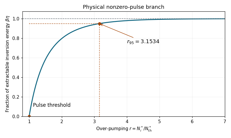

Extracting 95 percent of the maximum available inversion energy means , or . Substitution in ii givesThe degeneracy factor cancels because the target is a fraction of the maximum energy , rather than a fraction of without that factor.
During the pulse, the photon density reaches its maximum when with , so . Evaluating i at this inversion givesThe ideal instantaneous output power is . ThereforeFor , almost all the extractable energy is stored briefly as intracavity photons, and . The leading rise while the inversion remains near its initial value is , with short growth time . Depletion then takes the inversion below threshold. At late times andwhich approaches a tail with decay time at large . The pulse is consequently asymmetric, with a rapid rise and a slower approximately exponential trailing edge. The negligible-seed build-up delay depends on the seed strength. The pumping and spontaneous population decay have been neglected over the short pulse; parasitic cavity loss multiplies useful power by the output fraction described in ii.
For a paraxial Gaussian beam, choose the complex beam parameter withHere is the wavefront radius and the intensity radius. The ABCD law isFor a real, lossless round-trip ray transfer matrix in free space, . A reproducing cavity mode requires , henceExcept for a scalar identity matrix, a finite physical solution requires a complex-conjugate root pair, one with positive imaginary part. The generic strict stability condition is thereforeEquivalently, the ray eigenvalues are distinct unit-modulus numbers , so repeated round trips do not cause unbounded ray excursions. Adequate mirror apertures and longitudinal resonance are also needed for a low-loss resonant mode.
The strict inequality has a degenerate exception relevant to this paper. If , then for every physical even though . A symmetric confocal resonator has exactly this matrix and supports Gaussian modes; it is not excluded as a physical cavity. Thus the printed strict condition should be understood as the generic, nondegenerate stability criterion, not a universal necessary condition covering the confocal case in c.
Use the unfolded propagation convention after reflection. Free-space propagation and a concave spherical mirror have matricesThe mirror is equivalent in this paraxial convention to a thin lens of focal length . The excursion from the reference plane to mirror 1 and back isLikewise . Multiplying , or using cyclic invariance of the trace to move the reference plane, givesConsequently the strict criterion of a isThe trace is independent of , as a change of reference plane only conjugates the round-trip matrix. For the concrete confocal counterexample , , each excursion is and its square is . This gives and the degenerate boundary exception already explained.
Let , so each mirror in the symmetric confocal optical resonator has radius . At mirror 1, an incident beam whose waist is at the centre has , with distances measured along its incoming direction. Reflection givesAfter propagating the distance back to the centre, its parameter is purely imaginary. Thus the reflected waist is also at the cavity centre andThe incident and reflected waist radii need not agree. With axial position measured from the centre, their radii obeyAt either mirror, and the two spot sizes agree, as reflection requires. Between the mirrors they generally have different waists while still reproducing themselves after a full round trip.
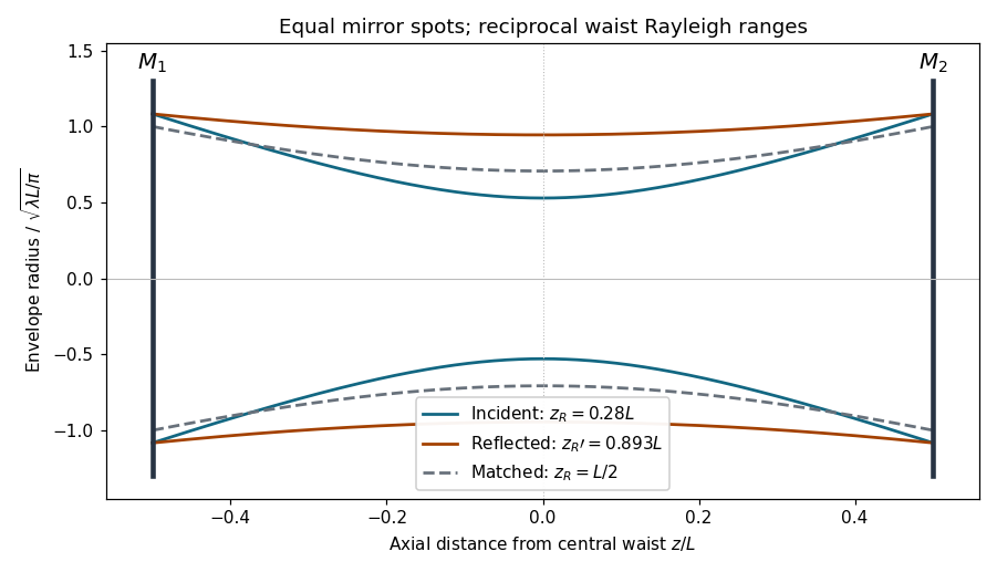

Equal waist sizes imply equal positive Rayleigh ranges, so c gives . Since , the matched radii areThese are radii; the corresponding spot diameters are twice these values. One practical disadvantage is the transverse-mode degeneracy of the exact confocal geometry: mode frequencies coincide in families, making clean selection of a single transverse mode more difficult. Its condition also lies at the strict-stability boundary. For example, perturbing the two radii in opposite directions, and , gives for , an unstable perturbation. This does not mean that all perturbations, or the ideal confocal resonator itself, are unstable.
Let be the atomic levels, , and the annihilation operator of the single field mode. Choose the joint ground energy to be zero. The resonant Jaynes-Cummings model isThe first term counts field photons, the second the atomic excitation, and the interaction exchanges one photon for one atomic excitation. A phase redefinition makes real and positive. Resonance means ; the total excitation is conserved. Adding an overall constant gives the equivalent convention using and a zero-point field term.
The model follows from the electric-dipole interaction and the rotating-wave approximation, retaining the energy-conserving terms while dropping and . We assume a single quantized monochromatic mode and negligible cavity leakage and atomic relaxation over the time considered. With this convention, the resonant population Rabi angular frequency in the one-excitation subspace is .
Conservation of confines evolution from to . On this subspace,The interaction matrix squares to the identity, so its exponential separates into cosine and sine terms. The state isThe overall phase can be discarded or removed by the interaction picture. The relative phase follows from Schrödinger evolution with the positive coupling in a. The atom and field are generally entangled; complete excitation transfer occurs at .
From b, the excited-state probability isFor a single short measurement interval beginning in , requiring before the first departure from unity givesA zero-photon outcome resets the conditional state to . After such tests, the probability of the all-zero-photon record isThus a 90 percent survival requirement over a specified total duration is stronger than the single-interval condition: approximately in the short-interval limit. The limiting preservation as is the quantum Zeno effect.
The measurement instrument matters. If photons are absorbed and their first detection removes the excitation, this survival probability also equals the unconditional excited population. For ideal nondestructive photon-number measurements, excitation can transfer back after a one-photon result; the unconditional result after equal intervals is instead . It also tends to one for fixed as the intervals shrink. Neither interpretation guarantees indefinite 90 percent survival merely by imposing a 90 percent bound on each separate interval.
There is at most one field photon in b. Projection onto its one-photon sector givesBefore detector absorption, the normalized conditional joint state is up to an overall phase. A destructive photon count changes the field to its vacuum but leaves the atom in . This conditional state is meaningful whenever the one-photon outcome has nonzero probability.
Discarding the photon-number result gives a classical mixture of the two outcome branches. The atomic state, in the basis , isIt is also the reduced state before measuring the field; a nonselective operation on the field does not change the atomic reduced density matrix. The atom is not in a coherent superposition with these populations.
For an atomic energy gap , the thermal population ratio is . Matching it givesA finite positive temperature exists when , with at and as from below. Equal populations correspond to zero inverse temperature. If , the expression is a negative effective temperature for a bounded two-level system, not an equilibrium state at any ordinary positive temperature. For a concrete counterexample to an unrestricted positive-temperature interpretation, at the atom is certainly excited, whereas every positive-temperature Gibbs distribution has . The fully excited endpoint is the formal limit . Matching one density matrix does not establish genuine thermalization with a bath.
Alice conditions on her observed computational-basis result. For outcome , occurring with probability , her post-measurement density matrix is ; for outcome , occurring with probability , it is . Explicitly,These are the conditional Lüders rule updates for the two rank-one projectors. They assume the corresponding outcome has nonzero probability and Alice knows which one occurred.
Bob knows the initial amplitudes and the measurement basis but not its result, so he averages the two conditional states:The initial matrix had off-diagonal entries and , which the unread measurement removes. Alice's description is conditioned on an available record; Bob's is the nonselective projective measurement mixture. Averaging Alice's records gives exactly Bob's predictions, and communicating the result lets him make the same conditional update. This is a difference of conditioning information, not two inconsistent physical state assignments.
Apply a Hadamard gate before a Z-basis measurement: and . The result probabilities areFor measurement statistics the network is followed by . If the measured qubit survives and should be left in the original X eigenstate, append a second after the nondestructive . The resulting instrument has Kraus operators and , not Z-eigenstate outputs.
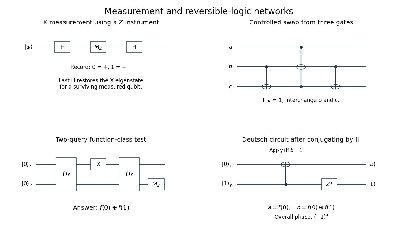
Original networks for X measurement, a controlled swap, two-query parity testing, and the simplified Deutsch circuit
. Time runs left to right. Filled controls and circled targets denote computational-basis controlled-NOT operations. In the last network and ; powers zero omit a gate. Details.
Bob must discard both results. An unread X measurement gives . Each of these two X eigenstates gives Z outcomes with probabilities . The final unread Z measurement therefore givesEquivalently, in the Bloch-vector description the first measurement retains only the X component, and the second retains only the Z component, leaving none. The final state is independent of the original .
Use the fidelity between the original pure state and the measurement output averaged over Calvin's results. Put , so . The output is , andHere is the input Bloch component. If a particular result is specified instead, the conditional fidelities are and ; their outcome-weighted mean is precisely the displayed . This distinction fixes what is meant by the fidelity of the measurement procedure.
Since with , its maximum occurs at or :up to a global phase. These are the eigenstates of the measured observable, so their ideal measurement does not disturb them.
Complete the square: . ThereforeEvery equatorial Bloch-sphere state attains the minimum, not just and . Its unread Z measurement gives , having removed all information contained in its relative phase.
For a uniformly distributed pure qubit on the Bloch sphere, rotational symmetry gives . ThusEquivalently, is uniform on under this measure and . The three positive coordinate-axis states mentioned in the source give , , whose average is the same because this fidelity depends only on the quadratic component . This is a specified uniform-state average, not a statement about every possible prior ensemble.
Assume Alice independently chooses X or Z with equal probabilities and that bit labels identify the corresponding positive and negative eigenstates. If Daisy measures Z, she reads a Z-encoded bit correctly with probability one and an X-encoded bit correctly with probability one half. ThereforeThe probability to read the entire independently encoded -bit check number correctly by this strategy is .
Daisy's random choice of X or Z agrees with Alice's independent random basis with probability . Agreement gives the correct label with certainty and disagreement gives it with probability . Hencethe same result as a fixed Z measurement. Randomizing her basis does not supply the missing information about Alice's choice. These are the probabilities for the two specified strategies, rather than an assertion that they are optimal among all possible quantum measurements.
Alice verifies each submitted qubit in her recorded secret basis and checks its bit against the revealed number. For a forger who chooses X or Z at random and prepares the corresponding known-bit eigenstate, each bit passes with probability . With independent basis choices,The detection probability depends on Daisy's preparation strategy. The question does not restrict her to legitimate X/Z eigenstates. Once the bit is known, for bit zero the averaged acceptance operator isFor bit one it is . Both have largest eigenvalue . Preparing the corresponding eigenstate, a Bloch-vector bisector of the two candidate encodings, achieves this value; for bit zero it is .
The acceptance operator for the whole known check number is , whose largest eigenvalue is , so entangled preparation cannot improve this no-original-note optimum. Therefore unrestricted preparation instead givesThe random-basis value is the elementary protocol calculation; the second value states the best forging strategy allowed by arbitrary state preparation and no access to the original quantum note.
Yes, access to the original qubits can supply information about the secret encoding basis once the bit is known. For bit zero the possibilities are and , whose overlap is ; for bit one they are and with the same overlap magnitude. A Helstrom measurement for two pure states can identify which candidate was supplied more reliably than a blind basis guess. Measuring and preparing a state based on that evidence can improve an additional counterfeit, although the discrimination is not perfect and the measurement can disturb the original.
The no-cloning theorem rules out a deterministic perfect extra copy of both nonorthogonal candidates; it does not imply that access gives no advantage. The task of producing an additional accepted note should also be distinguished from simply returning the unaltered original, which already passes Alice's test. Requiring both the original and the extra note to survive imposes a further information-disturbance tradeoff.
Allow clean workspace bits, as in standard reversible computation. Boolean algebra expresses any Boolean function as XORs of ANDs and constants. A Toffoli gate maps to , so an initially zero target computes an AND without erasing the inputs. A CNOT gate accumulates XORs, and a NOT gate supplies complemented bits or constants. Intermediate products can be computed into workspace, XORed into an output, and then uncomputed by reversing the workspace computation. This realizes the reversible embedding for any Boolean function and, with reversible clean-up, universal reversible classical computation.
The Fredkin transformation has control and targets . A network of three gates, shown in i, iswhere the sequence is executed left to right. After the first gate ; after the second ; and the last gives . If , ; if , . Thus the circuit is exactly a Fredkin gate.
The workspace qualification matters for the unrestricted universality claim. On four or more wires, every embedded NOT, CNOT and Toffoli gate is an even permutation of all computational states. Without ancillary wires they cannot implement, for example, a permutation swapping just and while fixing the other four-bit strings. Clean ancillas remove this obstruction on the designated input subspace.
- : , constant.
- : , constant.
- : , balanced.
- : , balanced.
A two-query network begins in , calls , flips the input with , calls again, and measures the answer wire in Z. The successive states areThe measured answer is zero for constant functions and one for balanced functions. The circuit is drawn in i.
Explicit oracle circuits follow from the form :Thus the four circuits, respectively for the truth tables in i, are the identity on both wires; a NOT on the answer wire; a CNOT from input to answer; and a CNOT together with an answer NOT. The latter commute, so their order is immaterial. These circuits leave the input wire unchanged and XOR precisely into the answer.
Let be as in i. Insert the explicit oracle from ii between the two pairs of Hadamard gates. The network identitiesturn the entire network intoThis is the last simplified circuit in i. On the designated input , its reversed control is certainly one, soThe global phase is unobservable. Measuring the first wire therefore determines the function class with certainty after one oracle query, while the second wire returns to . These circuit identities are the network form of quantum phase kickback: the answer state between the Hadamards is the eigenstate , on which an XOR acts as a phase.
In a small trapped-ion quantum computer, use two long-lived internal states of each ion, for example a pair of hyperfine ground states or a narrow optical transition, as . Electric trapping fields confine a short ion string, laser cooling reduces its motion, and optical pumping initializes the internal states. State-dependent fluorescence supplies readout: one qubit level participates in a bright cycling transition and the other is dark.
A resonant microwave, Raman or optical drive performs a single-qubit Rabi rotation. The drive phase fixes a rotation axis in the Bloch equatorial plane and its pulse area fixes the angle; detuning or phase-frame control supplies Z rotations. Individual spatial or frequency addressing selects the intended ion.
For a two-qubit gate, couple internal states to shared quantized vibrational modes. Resolved motional sidebands let one ion's spin influence the collective oscillator and then the second ion's spin. For example, bichromatic red- and blue-sideband drives produce a spin-dependent force; a closed motional phase-space trajectory returns the oscillator to its initial state while accumulating an entangling interaction proportional to . Together with single-qubit rotations this implements a CNOT. The short chain has well-separated normal-mode frequencies, and sideband cooling and the Lamb-Dicke regime suppress unwanted motion and make coherent bus control practical.
As a single trapped-ion chain grows, it has more collective vibrational modes with increasingly crowded frequencies. A drive intended to address one motional sideband can excite nearby modes, leaving unwanted spin-motion entanglement and crosstalk. Resolving the modes requires longer or more carefully shaped gates, while heating and frequency drift become more consequential. Thus the shared motional bus that is simple for a few ions becomes difficult to isolate and return cleanly to its initial state for large registers. This is a control and scaling limitation, rather than a failure of qubits or gates to exist.
Use , . Choose the eigenstate phasesThe inverse relations are and . The X states are linearly polarized at and to horizontal, while the Y states have equal orthogonal amplitudes in quadrature and hence opposite circular polarizations. We define R as the state; descriptions as clockwise or anticlockwise must specify the observation direction and time convention.
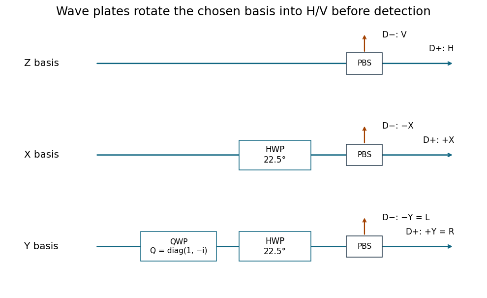
A polarizing beam splitter and two single-photon detectors directly measure Z, routing H and V to separate detectors. For X, place a half-wave plate with its axis at before that splitter; it implements a Hadamard transformation up to a global phase. For Y, first apply a quarter-wave retardance in the H/V axes and then the same half-wave plate. The total analyzer transformation is , with and . The physical fast/slow-axis assignment is selected to realize this stated retardance.

In ZZZ order, the only nonzero amplitudes are those of HHH and VVV. ThusFor an equatorial outcome , use the X and Y eigenvectors in a. For a product basis containing Y measurements, the bra acting on VVV contributes , while that acting on HHH contributes . Hence the amplitude of outcome in the supplied state isEach of XXY, XYX and YXX has , giving . In each of the three respective product bases,The eigenvector in each position belongs to the observable named in that position. All four outcomes with product have probability ; the four with have probability zero. This also specifies all eight probabilities in all three bases, and all single-site equatorial marginals are unbiased.
In a local hidden-variable description, assign predetermined values to the two possible measurements at photon . The perfect correlations of b requireMultiplying these identities cancels each squared X value and gives . Thus local realism predicts only the YYY outcomes and . Combining this parity rule with the measured unbiased single-Y marginals forces all four frequencies to be : four weights subject to normalization and the three zero-mean conditions are uniquely uniform.
Quantum mechanics instead has in the amplitude formula of b, giving . ThereforeQuantum mechanics predicts each positive-product outcome with probability and every negative-product outcome with probability zero. The local and quantum allowed sets are disjoint.
This is the GHZ theorem: in the ideal case the contradiction follows from deterministic product constraints, an all-versus-nothing argument. A usual two-party Bell-state test instead violates a statistical Bell inequality assembled from several settings. Both require appropriate locality and measurement-choice assumptions and careful treatment of experimental imperfections; the distinction is the deterministic form of the ideal three-party argument.
Write and . The ensemble is the mixture , rather than a coherent superposition of the two phases. The ZZZ probabilities stay unchanged. Reversing the relative phase interchanges the allowed parity sector in every equatorial basis, so for XXY, XYX and YXX,In YYY the quantum prediction is the opposite:For a concrete continuation of the ideal local analysis, apply the same phase-flip event to a predetermined local assignment: it reverses X and Y at the affected photon. All three mixed-basis products and the YYY product then reverse together. With unbiased marginals in each parity sector this shared-error local model predicts negative-product YYY outcomes at each and positive-product outcomes at each. The histograms compare this specified model with the quantum result.
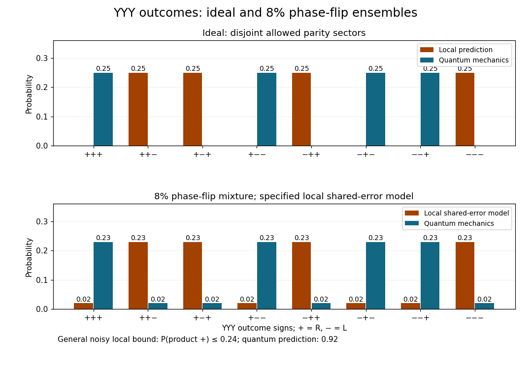

Imperfect mixed-basis statistics alone do not force that particular local histogram. A model-independent constraint follows because a positive YYY product requires at least one of the three ideal mixed-product constraints to fail. Each fails with probability , so the union bound givesEquivalently, local assignments satisfy , whereas this noisy quantum state gives . Thus the violation survives the specified phase error without assuming a unique noisy local histogram or independent errors in the three measurement contexts.
Articles by others on the same topic
There are currently no matching articles.