After division by , the linear ordinary differential equation becomesThe integrating factor is . ThusThe initial condition gives , so
Use reduction of order: set , so and . Substitution and cancellation giveSince , this reduces to , hence and . The general solution isThe two solutions are linearly independent, since their ratio is nonconstant; equivalently, their Wronskian is .
The homogeneous linear differential equation has general solution . For a particular solution, use variation of parameters with , and Wronskian one:The double-angle formulas and integration by parts giveSubstitution simplifies to . Absorb the last term into the homogeneous linear differential equation solution. ThereforeIndeed, applying to gives , and applying it to gives ; their difference divided by four is the required .
In Cartesian coordinates, a parametrization of the curve isDifferentiate using the product rule:Squaring and adding cancels the mixed terms, giving . The arc length is the integral of the speed, soThis assumes the parametrization is piecewise continuously differentiable and counts length with multiplicity if the curve is retraced.
The cardioid has reflection symmetry about the axis because . It passes through at , through at , and has a cusp at the origin when . These points and the following sketch show its orientation.
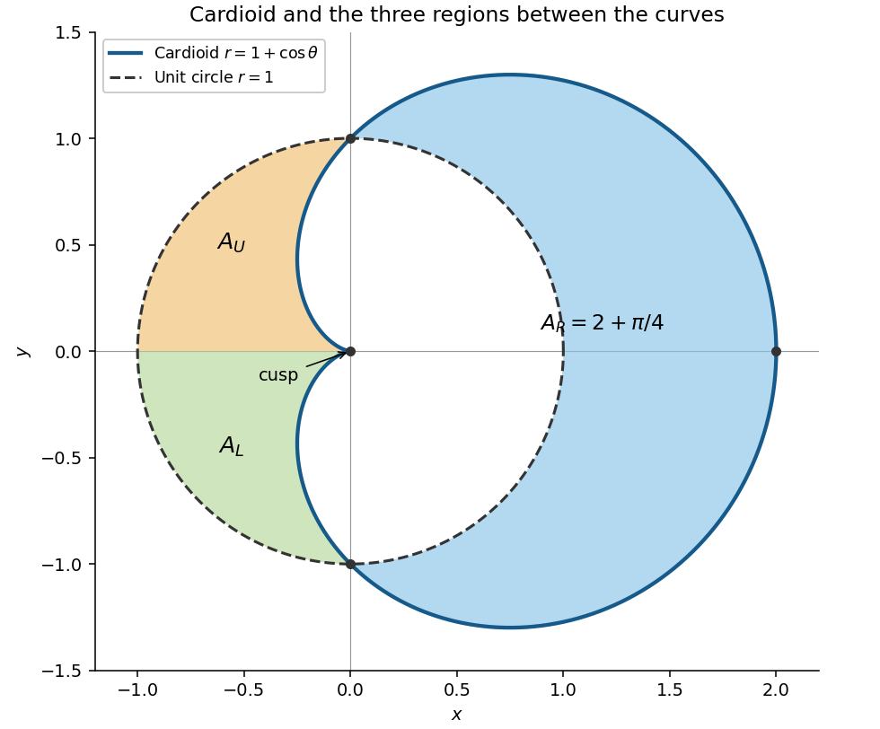
The cardioid and unit circle, with the three regions between them shaded
. Details. 
The cardioid meets the unit circle where , namely at . The polar area formula gives the area between radii as .
For , the cardioid lies outside the unit circle. The right-hand region therefore has areaOn , the unit circle lies outside the cardioid. The upper left region has areaBy reflection symmetry the lower left region has the same area. ThusThe two left regions touch only at the cusp; their interiors are disconnected. As a check, the difference between the cardioid's total area and the unit circle's area is .
Write , , and let , and be evaluated at the critical point. Assuming is twice continuously differentiable nearby, the Taylor expansion isThe linear terms vanish because the gradient is zero. For , completing the square givesConsequently the requested constant is the Hessian determinantThe displayed identity in the question is an identity for the quadratic part; for a general , its right-hand side needs the remainder .
If , the quadratic form is positive for every nonzero . On the unit circle it has a positive minimum, so it dominates the remainder sufficiently near the critical point. Hence the point is a strict local minimum.
If , along the quadratic term is , whereas along it is . Along each line the remainder is of smaller order. Thus values both above and below occur arbitrarily nearby, giving a saddle point.
The Hessian matrix and Hessian determinant areAt , , so this is a saddle point. At , and , so this is a strict local minimum. ThereforeThe value at the local minimum is ; there is no local maximum.
Let and . The unit sphere is compact, so the continuous function has a global maximum and global minimum. Since on the unit sphere, all such points satisfy the Lagrange multiplier equationsThus and either or .
Put . Since takes positive integer values, . Taking differences of the given tail probabilities therefore yields, also for ,This is the probability mass function of the geometric distribution on .
The mean is the derivative at one of the probability generating function. ThereforeEvaluation at one is valid here because the probability generating function has radius of convergence .
The event occurs exactly when both and . By independence,ThusThe new success probability is the chance that at least one of the two trials succeeds.
Since , its finite mean satisfies . Every is nonnegative, andThus is a probability mass function. It defines the size-biased distribution of : an outcome of size receives times its original relative weight.
By the definition of a probability generating function,Termwise differentiation of the power series is valid for . At , the equality extends by the finite mean assumption, and both sides equal one.
For the geometric distribution, , so the probability generating function of the size-biased distribution isIf are independent and identically distributed with geometric distribution of parameter , the probability generating function of an independent sum givesAt zero, interpret the expression by its continuous extension. The probability generating functions agree, henceOne can also check the probability mass functions directly: for , there are positive integer pairs with sum , each having probability . Thus both sides assign probability to .
A partition of a set is a collection of nonempty subsets whose union is and which are pairwise disjoint:For use with probabilities, the must also be events in the sample space.
For a finite or countable partition of a set into events , the law of total probability statesThe events are pairwise disjoint and have union , so countable additivity proves the formula. Terms with contribute zero and are omitted to avoid undefined conditional probabilities.
There are two paths from back to in two steps: and . By the markov property, their probabilities multiply along each path. Therefore
Let . The law of total probability applied to the current markov chain state givesThe second equality holds because can only be reached from . Eliminating gives the linear recurrence relation
The characteristic equation of a linear recurrence isIts distinct roots are and , so . The initial conditions are and , giving and . Hence , , and
Starting from at time , the markov property and the time-independent transition rules give . ThereforeWrite . The conditional probability becomesThe conditioning selects paths which have avoided the absorbing state up to time ; it is therefore quite different from the unconditioned probability , which tends to zero.
For the rate-one exponential distribution, the probability density function is for . By integration by parts,Thus
The products and share , so they are not independent. Using the definition of covariance and the independence of ,By contrast, and depend on disjoint sets of independent random variables, so they are independent and have zero covariance. Hence
Assume finite second moments and write . Expanding the square in the definition of variance givesRecognizing the two variances and the covariance, we obtain
For random variables with finite second moments, the variance of a sum isNo independence assumption is needed.
Write , so . Each product has mean one, and its variance isAdjacent products share one factor, giving covariance one by part (a)(iii). Products whose indices differ by at least two involve disjoint independent random variables, so their covariance is zero. There are adjacent pairs. By the variance of a sum,
By Chebyshev's inequality and part (i),This actually proves the stronger statement , namely convergence in probability, despite the statistical dependence between adjacent products.
Let . For an observed sample in the nonnegative orthant, the likelihood function under the uniform distribution isIt is zero for , and decreases with on . Thus the maximum likelihood estimation problem is solved at the smallest admissible value:Under the model with probability one. The all-zero sample is a null event on which the likelihood function has no finite maximizer in the parameter space .
For , independence and the uniform distribution giveTherefore the cumulative distribution function isIt contains no , so is a pivotal quantity.
Differentiating the cumulative distribution function in part (ii) gives the probability density function on . HenceThus an unbiased estimator based on the sample maximum is
Each observation from the uniform distribution has mean . By linearity of expectation, , so another unbiased estimator is
The pivotal quantity lies in and satisfies . ThusRearranging these inequalities yields the exact confidence intervalFor every , its coverage probability is exactly ; the result uses the finite-sample probability distribution, with no normal approximation.
The log-likelihood function for the Laplace distribution isThus maximum likelihood estimation is equivalent to minimizing the sum of absolute values. Write and sort the data as . Between observations, if values lie to the left of , the derivative of is . It is negative before the middle observation and positive after it. The minimum occurs at the sample median:This minimizer remains unique for odd even when some observations coincide, since fewer than half the observations can lie strictly on either side of the middle value.
Treat the explanatory variables as fixed and put , . To identify both slopes, assume and . The given centring and orthogonality conditions make the three columns pairwise orthogonal.
The log-likelihood function in the normal linear model, up to a constant independent of the coefficients, isThus maximum likelihood estimation minimizes the residual sum of squares. Setting its partial derivatives to zero givesUsing decouples these equations:The Hessian matrix of the residual sum of squares is , which is positive definite. These are therefore the unique minimizers. If either squared sum is zero, the associated explanatory variable vanishes identically and its coefficient cannot be identified.
Substitute the linear regression model into the estimators and use the centring and orthogonality conditions:A linear combination of independent normal random variables is normal. Their means are and , while variance additivity for independent random variables givesConsequently
The central limit theorem states that if are independent and identically distributed with finite mean and variance , thenHere denotes convergence in distribution.
The algebraic identity does not require a normal distribution for the errors. Applying the central limit theorem to their sample mean givesThus, for large ,Its mean and variance remain exact, even though its normal distribution is now only an approximation. With the error probability distribution unspecified, the formula is retained as an estimator; it is not being asserted to remain a maximum likelihood estimation formula.
No, not from the stated assumptions alone. The centered slope is a weighted sum,and the weighted errors need not be identically distributed. The ordinary central limit theorem therefore does not apply directly.
For a concrete counterexample, for every chooseThese satisfy all three centring and orthogonality assumptions, and both explanatory columns are nonzero. Let the errors be independent with Rademacher distribution, taking values with equal probability. Thenwhich takes values with probabilities for every . Increasing the sample size adds no information about this slope, and the standardized estimator does not approach a normal distribution.
A useful additional assumption for asymptotic normality of a weighted regression slope is that no single design value dominates:Under this condition and the given finite error variance, the Lindeberg-Feller central limit theorem yieldsjustifying the approximation for the slope as well.
Articles were limited to the first 100 out of 105 total.
Articles by others on the same topic
There are currently no matching articles.