Three vectors in three-dimensional Euclidean space are non-coplanar precisely when their scalar triple product is nonzero. Put . In particular, . The identity for cross products with a common vector givesFor completeness, this follows from the vector triple product identity: writing gives , with and . Therefore the new scalar triple product isThus are non-coplanar, or equivalently linearly independent.
Take the dot product of the equation with . Since , we obtain . Next take its cross product with and apply the vector triple product identity:Substitute and the known dot product, then rearrange:Here the vectors and are real, so the denominator is positive. The formula also covers , giving . To check existence as well as uniqueness, write its numerator as . The vector triple product identity gives , so . Substitution verifies the original equation. This is an instance of the inverse of a scalar plus a cross-product operator.
Let be the given integral. Its integrand extends continuously to , with value . The Leibniz integral rule includes both the moving upper endpoint and the derivative of the integrand. For it givesConsequentlyThe zero case follows directly from near zero: expand and integrate up to . Equivalently, the change of variables gives , whose derivative is the same expression, interpreted continuously at zero. This substitution works for negative as an oriented integral too.
Use the complex exponential representation of cosine. For real and , exponential decay makes the improper integral absolutely convergent, andFor the second integral, use differentiation under the integral sign with respect to . The minus sign is essential: . HenceTo justify this step near any fixed , restrict . The absolute value of the differentiated integrand is at most , an integrable bound, so dominated convergence permits the differentiation. At the answers reduce to and , respectively.
Use spherical polar coordinates with measured from the positive axis and around that axis:The standard full-space ranges are , , . The factor is the absolute Jacobian determinant and gives the volume element.
The mass density becomes . Integrate it over the sphere using the spherical polar coordinates and volume element above:The angular integral is , since . ThereforeThe term proportional to contributes zero by reflection across the equatorial plane. Thus the answer is also the volume times the average mass density . The undefined direction at the origin affects a single point and has no effect on this volume integral.
In the first octant, spherical polar coordinates have and . The charge density is . Hence the total electric charge isThe three factors are , , and , respectively. For the middle integral, set to obtain . Thus
The number of successes has a binomial distribution. Each arrangement of successes and failures has probability by independence, and the binomial coefficient counts the arrangements. ThereforeThe final equality is the binomial theorem. Writing as a sum of independent Bernoulli random variables gives its expectation and variance: , . Thus the matching normal distribution hasThe normal approximation is appropriate when both expected counts and are sufficiently large; large alone is insufficient if is extremely close to zero or one.
For the guessing student, , , . Therefore the expected number of correct answers is , and , . The inclusive integer range becomes after the continuity correction. Standardizing the normal distribution givesHere , and the last step uses the supplied bound. The approximate probability is . The normal approximation provides the requested conclusion; as a separate check, summing the five exact binomial probabilities gives approximately , also exceeding one half.
The required matrix form of the linear system isSubtract the first row from the third and expand the determinant along the resulting row:Thus the linear system has a unique solution, for every real , precisely when .
For , the second equation gives . Subtracting the first equation from the third gives , and the first equation then determines :For , the first and third left-hand sides are identical but their right-hand sides are and . HenceFor , subtracting the first equation from the third gives . The first equation now gives , while the second requires . ConsequentlyThe free variable in a linear system in the consistent singular case describes a line of solutions. These direct reductions distinguish an inconsistent linear system from one with infinitely many solutions, which a zero determinant alone cannot do.
Compute the curl component by component from the given vector field:For example, and . Its divergence isas expected because the divergence of a curl is zero.
Take counterclockwise when viewed from positive , the disc upward oriented, and the hemisphere outward oriented. These choices give both surfaces the same positive boundary orientation. Parametrize by , . On it, and , so the line integral isOn , use polar coordinates and . Since there, the surface flux isOn the unit hemisphere, the outward unit normal vector is . Since , we have . In spherical polar coordinates, and , giving the explicit surface integralIndeed the inner integral is .
These equalities illustrate Stokes theorem twice: and either upward or outward spans the oriented circle , so each surface flux equals the same line integral. For the divergence theorem, close the upper half-ball by adjoining the downward oriented base, namely . Its outward surface flux isThe minus sign on the base is required because its outward normal vector points down. Reversing a specified orientation reverses that integral's sign.
The characteristic equation of the associated homogeneous linear ordinary differential equation is , so the complementary function is . For a particular solution, try . Substitution gives , so , . The unrestricted solution is thereforeIts derivative at zero is . The single prescribed condition imposes and leaves one arbitrary constant. Thus the most general permitted solution isThere is no condition fixing , so the remaining arbitrary constant is essential.
Write with . By the chain rule,The terms involving cancel in the original ordinary differential equation, leavingOn each interval where , the transformed linear ordinary differential equation is . Its characteristic equation has roots , yieldingDirect substitution shows these expressions also extend smoothly through and satisfy the original equation there. The two constants describe the general solution on any interval where the coordinate substitution is invertible.
An orthogonal matrix satisfies , while a symmetric matrix satisfies . Combining them gives . For the product with the antisymmetric matrix , the rule for the transpose of a matrix product givesThus is an antisymmetric matrix exactly when . The hypotheses do not force this commutativity. For a counterexample, takeHere is a symmetric matrix and an orthogonal matrix, and is an antisymmetric matrix and an orthogonal matrix, but is a nonzero symmetric matrix, so it is not an antisymmetric matrix. On the other hand, the product of two orthogonal matrices is always an orthogonal matrix:Therefore the answers are
Call the given matrix . Its middle coordinate decouples, immediately giving the eigenvalue with normalized eigenvector . The remaining characteristic polynomial comes from the block:For , the first row of gives ; for , the first row of gives . After vector normalization, one possible complete set isEach has unit Euclidean norm. The dot products with vanish because the other two middle components are zero, and . This explicitly verifies orthonormality, also predicted by the spectral theorem for real symmetric matrices with distinct eigenvalues. Changing any eigenvector's sign gives an equally valid normalized choice.
The Taylor expansion about has coefficients given by the successive derivatives at :When is times continuously differentiable on the interval between and , Taylor's theorem gives for an intermediate point . If the remainders tend to zero, this yields the infinite Taylor series . The three functions below are real analytic near zero after taking the continuous extension in part (i).
First expand the exponential function and divide by :Seek its reciprocal as . Equating coefficients in the product with this expression givesHence , , . The first three nonzero terms of the Taylor expansion areAlthough the quotient is undefined at zero as written, its limit is one, and this Taylor expansion belongs to its continuous, real analytic extension.
Let . The derivative identity for tangent gives , so , , and . Its first three nonzero Taylor expansion terms are thereforeThe factor on the second derivative is what turns into the coefficient .
Use and . To obtain enough terms of tangent, write ; it is an odd function. The identity givesso , . Integrate this Taylor expansion term by term from zero to :There is no constant term, and only even powers occur because is an even function near zero. Thus reaching the first three nonzero terms requires expansion through degree six.
The comparison test for series states that if for all sufficiently large , then convergence of implies convergence of ; conversely, divergence of implies divergence of . A summable bound on proves absolute convergence of .
For the ratio test, suppose the terms are eventually nonzero and exists. If , the series converges absolutely. If , including , the terms fail to tend to zero and the series diverges. If , the test is inconclusive. An eventually zero series converges separately. Convergence means that the sequence of partial sums has a finite limit; the terms tending to zero is only a necessary condition for a convergent series.
For every real , . The bounding P-series with exponent two converges. The comparison test for series therefore givesOscillations of cosine are unnecessary for convergence here.
This is a geometric series with ratio . Since , the condition is equivalent toIt holds for every real except . At the terms are all one; at they alternate between and . Neither sequence of terms tends to zero. ThusAll the convergent cases have absolute convergence, including , when every term is zero.
For , the ratio test givesThis is less than one exactly when . For the terms are , and for they grow exponentially; in both cases they fail to tend to zero. Consequently
Rationalize the difference to reveal its small size instead of comparing its two large summands separately:For any fixed real , the right-hand series is a constant multiple of a convergent P-series. The comparison test for series provesThe case is the identically zero series. For nonzero , its summand is asymptotic to , explaining the same convergence behavior as the inverse-square series.
The coordinate partial derivatives are , , , and . Apply the multivariable chain rule to :All partial derivatives of are evaluated at . This is a logarithmic polar coordinate change; its Jacobian determinant is , so it is locally invertible away from the origin. A full angular turn repeats the same point, as usual for polar coordinates.
Differentiate with respect to , remembering that its coefficients also depend on . The product rule and multivariable chain rule giveFor a twice continuously differentiable , equality of mixed partial derivatives gives . HenceThe first-order terms come from differentiating and themselves; treating as an operator with constant coefficients would miss them.
The last two terms in the preceding result equal . ThereforeThe left-hand side of the original partial differential equation is consequently , givingIn these variables it has the form of a heat equation, with logarithmic radial coordinate playing the evolution variable and angular coordinate playing the spatial variable. If is single-valued around the whole punctured plane, then as well; that periodicity is a global coordinate condition, not an extra local transformation term.
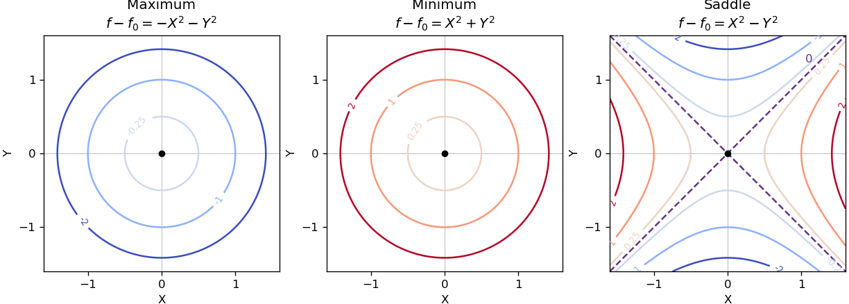
Near a nondegenerate stationary point, the quadratic part of the Taylor expansion determines the local contour plot. For a strict local maximum, the model gives nested closed level sets, with values decreasing as one moves outward. For a strict local minimum, the model gives the same nested shape with values increasing outward. Unequal nonzero quadratic coefficients stretch the circles into ellipses after a rotation to the Hessian matrix's eigenvectors.
For a nondegenerate saddle point of a scalar function, the model gives hyperbolas. Levels above open along the positive-curvature direction; levels below open along the negative-curvature direction. The critical level set is the two crossing lines . Degenerate stationary points can have different local geometry, so these are the standard nondegenerate sketches.

Set both first partial derivatives equal to zero:Thus and , independently, giving exactly nine stationary points. The Hessian matrix is diagonal everywhere:Its diagonal entries are its eigenvalues, so the second-derivative test immediately classifies the points:
- At , the Hessian matrix has eigenvalues . These two points are strict local maxima, each with .
- At , the Hessian matrix has eigenvalues . These two points are strict local minima, each with .
- At , the Hessian matrix has eigenvalues , so it is a saddle point of a scalar function with .
- At , with all four sign combinations, the Hessian matrix has eigenvalues . These four points are saddle points of a scalar function, each with .
In particular,All nine stationary points are nondegenerate, so no higher-order test is needed. Neither type of local extremum is global: as , whereas as .
To organize the contour plot, complete the squares:The level set through all four outer saddle points of a scalar function factors exactly:It is therefore the union of the circle and the hyperbola , which cross at those four saddle points of a scalar function. Near the origin, , so the zero contours have tangents . These two exact structural features, together with the nested contours around the four local extrema, determine the requested sketch. They are an example of a separable quartic landscape with nine stationary points.
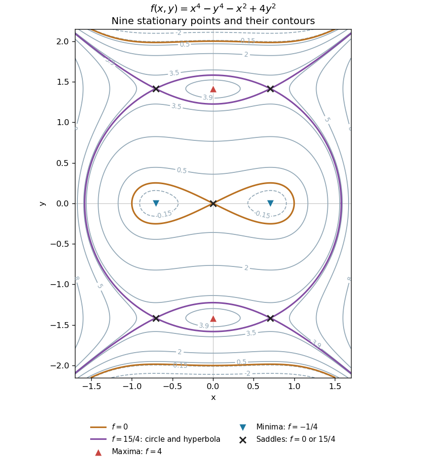
All nine stationary points and contours of the separable quartic
. Original contour plot of . The two maxima, two minima and five saddles are marked. The exact level is highlighted as a circle and a hyperbola intersecting at the four outer saddles; the zero contour crosses at the origin. Details.
Articles by others on the same topic
There are currently no matching articles.