Past exam of the mathematics course of the year 1 of the natural sciences course of the University of Cambridge / 2013 / Paper 2

The two dot products are $\mathbf{a}\cdot \mathbf{b}=2-1-6=-5$ and $\mathbf{b}\cdot \mathbf{c}=-1-3=-4$. Therefore

The cross product is $\mathbf{a}\times \mathbf{b}=(1,-7,-3)$. Taking its dot product with $\mathbf{c}$ gives the scalar triple product

The defining exponential function formulas for the hyperbolic functions give

For a real number $x$, the hyperbolic functions satisfy $\cosh x>0$ and $1-{\tanh }^{2}x={\mathrm{sech}}^{2}x$. Hence $\cosh x=1/\sqrt{1-u^2}$, and multiplying it by $\tanh x=u$ givesThe sign of the numerator preserves the sign of $\sinh x$.

Multiply numerator and denominator by the complex conjugate of the denominator:Thus the real part and imaginary part are $\boxed{\mathrm{Re}=-5/13,\mathrm{Im}=-12/13}$.

The gradient is $\nabla \varphi =(2xy+z,x^2,x)$, with value $(3,1,1)$ at the point. Normalize the direction to a unit vector: $\hat{\mathbf{s}}=(2,0,1)/\sqrt{5}$. The directional derivative is therefore

The characteristic polynomial is $(1-\lambda )(4-\lambda )-4=\lambda (\lambda -5)$. Solving each eigenvalue equation gives the eigenvalues and eigenvectorsFor unit-length representatives divide each displayed direction by $\sqrt{5}$. The two eigendirections are orthogonal, consistently with the matrix being a symmetric matrix.

Put $h=x-\pi /4$. The trigonometric identities give $\cos x\sin x=\frac{1}{2}\sin 2x=\frac{1}{2}\cos 2h$. Expanding cosine at zero givesThe linear and cubic terms vanish, so these are the first two nonzero Taylor series terms.

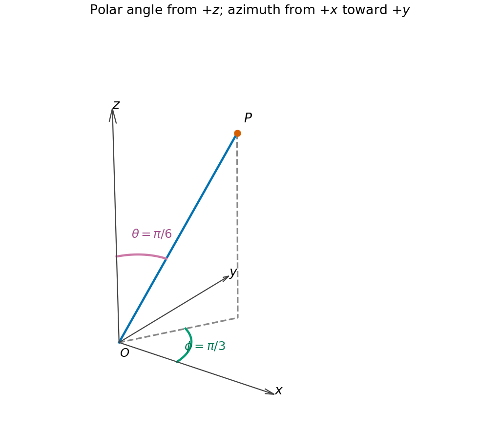
Use the convention that $\theta$ is the polar angle from positive $z$, and $\varphi$ the azimuth from positive $x$. The radius isThen $\cos \theta =z/r=\sqrt{3}/2$, while $\tan \varphi =y/x=\sqrt{3}$ and both planar coordinates are positive. Thus the spherical coordinates are

Project the radius vector onto the $x$-$y$ plane. The polar angle $\theta =\pi /6$ lies between the positive $z$ axis and $OP$. The azimuth $\varphi =\pi /3$ lies in the $x$-$y$ plane between the positive $x$ axis and the projection of $OP$, measured toward positive $y$.

First take $F_y=x{e}^{\sin (xy)}\cos (xy)$, then differentiate with respect to $x$. The product rule and chain rule giveThe function is smooth, so the two mixed partial derivatives agree.

For the divergence in Cartesian coordinates, differentiate each component with respect to its own coordinate:The third component contributes zero because it is independent of $z$.

For $r>0$, use the gradient of a radial function with $g(r)=1/r$:Equivalently each component is $-x_j/r^3$ by differentiating $r^2=x^2+y^2+z^2$. The origin is excluded from the function's domain.

The product rule for divergence, $\nabla \cdot \mathbf{r}=3$, and the result in (a) give, for $r>0$,This is a pointwise identity away from the origin, where the radial unit vector is undefined.

For independent events from fair dice, the probability of a six on each roll is $1/6$. Multiplication gives

The complement of an event here is that all three dice avoid six, with probability $(5/6{)}^3$. Therefore

The probability density function is nonnegative for $\alpha >0$. Its integral over the support isso it is normalized for every $\alpha >0$. This is the unit-threshold Pareto distribution.

The expected value is the improper integral $\alpha {\int }_1^{\infty }{x}^{-\alpha }dx$. It converges exactly when $\alpha >1$, yieldingAt $\alpha =1$ this improper integral diverges logarithmically, and for $0<\alpha <1$ it diverges as a power of its upper endpoint. In both cases the nonnegative variable has infinite mean. This is the first Pareto moment threshold.

The second moment is $E[X^2]=\alpha {\int }_1^{\infty }{x}^{1-\alpha }dx$, finite exactly for $\alpha >2$, where it equals $\alpha /(\alpha -2)$. Subtracting the square of the mean givesFor $1<\alpha \le 2$, the mean exists but the variance is infinite. For $0<\alpha \le 1$, the ordinary centered variance is not defined because the mean is not finite. Thus there is no finite variance for any $\alpha \le 2$.

Integrating the probability density function from its lower endpoint to $x$ gives the cumulative distribution functionIt is continuous and strictly increasing on the support. Hence the unique median $m$ satisfies $F(m)=1/2$, or $m^{-\alpha }=1/2$. Therefore

The numerator event is contained in the conditioning event. The definition of conditional probability therefore givesThe denominator is positive for all $\alpha >0$, and endpoint strictness is irrelevant for a continuous probability distribution.

Using the Einstein summation convention, reorder the scalar components and sum over the two dummy indices separately:The repeated suffixes each represent the three-dimensional component sum.

Contract the Kronecker deltas in the first term to obtain $a_i{b}_i$. In the second term, ${\delta }_{ij}$ identifies the two $a$ components, while the two $b_k$ components already contract. Therefore

In three dimensions each contracted delta is the trace of the identity, ${\delta }_{jj}={\delta }_{kk}=3$. Thus the exponent is six and the base is $\mathbf{a}\cdot \mathbf{a}$. Hence

An antisymmetric matrix satisfies $A^T=-A$. Each diagonal entry is therefore its own negative, so both diagonal entries vanish. Consequently

A real two-dimensional antisymmetric matrix has the form $A=\left(\begin{array}{cc}0& s\\ -s& 0\end{array}\right)$. Its determinant is $s^2=1/4$, and the specified positive upper-right entry selects $s=1/2$. Thus

Direct multiplication gives $A^2=-I/4$. Therefore $A(-4A)=I=(-4A)A$, yieldingThe nonzero determinant ensures that this two-sided inverse is unique as a matrix inverse.

Multiply $A^2=-I/4$ by $A$ once more:No additional diagonalization is needed.

Repeatedly using the quadratic identity givesIn entries these are $(-1{)}^n{4}^{-n}\left(\begin{array}{cc}1& 0\\ 0& 1\end{array}\right)$ and $(-1{)}^n{2}^{-(2n+1)}\left(\begin{array}{cc}0& 1\\ -1& 0\end{array}\right)$, respectively. This is the basic reduction for functions of a two-dimensional antisymmetric matrix.

The even-power formula reduces every summand to a scalar multiple of $I$:Both series have absolute convergence. Apply the logarithm expansion ${\sum }_{n\ge 1}{z}^n/n=-\log (1-z)$ for $|z|<1$ to obtainThus the off-diagonal entries vanish and both diagonal entries have the required value.

Use integration by substitution with $x=2u$ and the Gaussian being an even function:The factor two from the differential exactly cancels the half-line factor in the given full-line Gaussian integral.

Retain the original PDF's full-line integration limits. For $n\ge 2$, write $x^n{e}^{-x^2}dx=-x^{n-1}d(e^{-x^2})/2$. Integration by parts givesGaussian decay dominates every power, so the endpoint term vanishes, soThis is the full-line Gaussian moment recurrence; its initial values differ from the half-line version.

The integrand for $I_1$ is an odd function with absolute convergence, so $I_1=0$. For $I_2$, the recurrence gives $I_2=I_0/2$, where the supplied Gaussian integral is $I_0=\sqrt{\pi }$. HenceThe zero first moment is specific to the symmetric full-line domain.

Use integration by substitution with the reciprocal variable $t=1/x$, so $dx=-dt/t^2$ and $\log x=-\log t$. The endpoints $x=1,\infty$ become $t=1,0$. ThusRenaming the dummy integration variable proves the identity without evaluating either side.

The integral converges absolutely: near zero it behaves like $\log x$, and at infinity like $(\log x)/x^2$. Let its value be $J$. The integration by substitution $x=1/t$ givesThereforeAbsolute convergence makes this cancellation between the two ends legitimate.

The tangent half-angle substitution $t=\tan (x/2)$ gives $\sin x=2t/(1+t^2)$ and $dx=2dt/(1+t^2)$. The endpoints become zero and one, soUse completing the square, $t^2+t+1=(t+1/2{)}^2+3/4$, and integrate:Thus both integrals equal $\boxed{\pi /(3\sqrt{3})}$.

The characteristic equation has roots zero and three, giving $y_h=C_1+C_2{e}^{3x}$. Since the forcing is quadratic and the homogeneous solution contains a constant, use the polynomial trial $y_p=A{x}^3+B{x}^2+Cx$. Substitution givesMatching coefficients gives $A=-1/3$, $B=-1/3$, and $C=-8/9$. Therefore

The common homogeneous solution is $C_1\cos 2x+C_2\sin 2x$. For forcing $\sin x$, a trial $a\sin x$ gives $3a\sin x=\sin x$, so the first general solution isFor forcing $\sin 2x$, the frequency produces resonance in a differential equation. A trial $ax\cos 2x$ gives $y_p^{\prime \prime }+4y_p=-4a\sin 2x$, so $a=-1/4$ and the second solution isThe superposition principle permits adding the two particular solutions. The sum-forcing equation therefore hasOnly one pair of homogeneous constants is needed, because the two original homogeneous families coincide.

Differentiate $y^{\prime }=-y+3x$ and use the other equation:Since $3x=y^{\prime }+y$, this becomes $y^{\prime \prime }-3y^{\prime }+2y=0$. Its roots are one and two, so $y=A{e}^t+B{e}^{2t}$. The given data imply $y^{\prime }(0)=-2+3=1$, hence $A+B=2$ and $A+2B=1$. Thus $A=3$, $B=-1$, givingRecover the other dependent variable from $x=(y^{\prime }+y)/3$:These expressions satisfy both original equations and the two initial values.

The Euclidean distance is $D(x,y)=\sqrt{x^2+y^2}$. Along the parametric curve,This is at least $a^2$, with equality exactly when $t=0$. Therefore

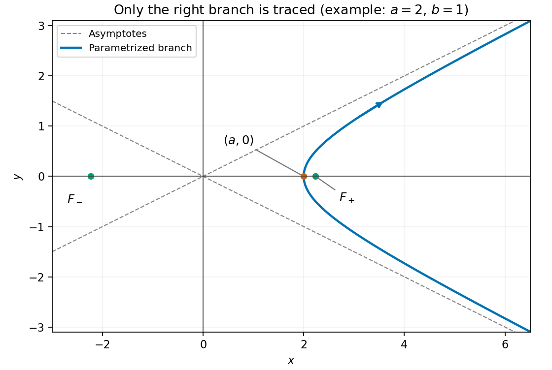
The hyperbolic functions identity eliminates $t$ from the parametric curve:The restriction is essential: $\cosh t\ge 1$, so the parametrization traces only the right branch of the full hyperbola. Conversely, every point on that right branch is reached by taking $t=\mathrm{arsinh}(y/b)$.

Solving for $y$ gives $y=\pm (b/a)\sqrt{x^2-a^2}$ with $x\ge a$. For large $x$, the square root is $x-a^2/(2x)+O(x^{-3})$, so the two asymptotes areThe curve lies between these lines on the right side and has its nearest point, with vertical tangent, at $(a,0)$. As $t$ increases it travels from the lower unbounded end through that vertex to the upper unbounded end. The left hyperbola branch is not part of the given curve.